Wavelet machine learning model for condition monitoring of ball bearings [version 2; peer review: 1 approved with reservations, 1 not approved]

Дата публикации: 27-07-2026 05:36:53

This research presents an integrated condition monitoring framework for deep groove ball bearings by combining Complex Morlet Wavelet (CMW) analysis, machine learning techniques, thermographic analysis, and SKF Machine Condition Advisor tools. The proposed methodology employs Fast Fourier Transform (FFT) and Complex Morlet Wavelet-based vibration signal processing to extract discriminative time–frequency features for the early detection and diagnosis of bearing faults under both single and combined fault conditions. To evaluate fault classification performance, three machine learning algorithms, namely Artificial Neural Networks (ANN), Support Vector Machines (SVM), and Random Forest (RF), are implemented and comparatively analyzed. Experimental investigations are conducted on a laboratory-scale bearing test rig operating under controlled conditions. The extracted wavelet-based features effectively characterize fault-induced vibration signatures, enabling accurate fault identification and classification. Comparative results indicate that Random Forest achieves the highest classification accuracy, followed by SVM and ANN. The average classification accuracies obtained using RF, SVM, and ANN are 97.48%, 95.27%, and 87.20%, respectively, demonstrating the superior robustness and generalization capability of the ensemble learning approach. Furthermore, thermographic analysis and SKF Machine Condition Advisor measurements provide complementary information for validating fault severity and machine health conditions, thereby enhancing diagnostic reliability. Although the present study is limited to constant-speed operation and controlled laboratory environments, the proposed framework demonstrates significant potential for predictive maintenance and intelligent condition monitoring applications. The integration of advanced time–frequency analysis, machine learning-based fault classification, and practical condition monitoring tools offers an effective and reliable solution for machinery health assessment in industrial environments.

Основное содержимое страницы с новостью.

Revised Amendments from Version 1

This article is a substantially revised and extended version of our previously published work. The current version includes a more comprehensive experimental investigation of bearing fault diagnosis using Complex Morlet Wavelet-based time–frequency analysis. In addition to the Artificial Neural Network (ANN) and Support Vector Machine (SVM) classifiers presented earlier, the revised manuscript incorporates a Random Forest (RF) classifier and provides a detailed comparative evaluation of all three machine learning approaches. New experimental results, performance metrics, and classification analyses have been added to demonstrate the effectiveness of the proposed framework under various single and combined bearing fault conditions.
Furthermore, the manuscript has been expanded with enhanced discussions on vibration signal processing, thermographic analysis, and SKF Machine Condition Advisor-based condition monitoring. Additional figures, tables, and performance comparisons have been included to improve the clarity and completeness of the study. The results show that the Random Forest classifier achieves the highest overall classification accuracy, followed by SVM and ANN, thereby providing a more comprehensive assessment of intelligent fault diagnosis techniques for bearing condition monitoring. These additions significantly strengthen the technical contributions and practical applicability of the proposed predictive maintenance framework.

To read any peer review reports and author responses for this article, follow the "read" links in the Open Peer Review table.

1. Introduction

Reliability is a significant term related to the expected life of machinery and equipment. Better product design has a significant impact on the life or reliability of a product.^1,2 Although the product has a better design, the real operating conditions impart variable stress and load, which deteriorates the product over time. Hence, maintenance is the only key to achieving an acceptable consistency level. The condition-based maintenance procedure or the preventive maintenance procedure is widely used to eliminate excessive repair work by implementing the repair schedule, only when there is a warning of unusual performance of the appliance or the element.³ This maintenance activity is based on the data gathered from various condition-based procedures. In this recent era, condition monitoring and fault analysis of rotating and reciprocating machineries are the subjects of interest among researchers who aim to increase the reliability and safety of machineries.⁴ Shaft and bearing failures are considered to be the main reasons for the failure of revolving and reciprocating machineries.⁵ During operation, the conditions of the shaft and bearings continuously change. Hence, the vibration signals and other process parameters also changed continuously. These characteristic features of shafts and bearings enable vibration analysis and other condition-monitoring techniques.⁶ Several studies have been conducted to investigate the health of bearings and attached shafts. Of these non-destructive techniques (NDT), vibration analysis, motor current signature analysis, acoustic emission (AE), sound level analysis, oil condition monitoring, and temperature monitoring techniques are found to be the most reliable methods.⁷ Vibration analysis techniques are frequently used in machine health monitoring. In this technique, a specific sensor called an accelerometer is used to sense the vibration signal, and the signal is processed using a Fast Fourier Transform (FFT) analyzer to specify and identify the position of the fault.⁸ In this recent era, researchers have used advanced techniques such as spectral kurtosis, Hilbert Huang Transformation, High-frequency resonance techniques (HFRT) and optimal wavelet-based methods to detect the precise position of the error in the rolling component bearing.⁹

Balls, cages, and inner and outer races are essential parts of rolling element bearings. Failure occurs in these components owing to pitting, bruising, etching, spalling, and wear. These are the outcomes of repeated and variable stresses, contaminated lubricants, excessive current and voltage, and the presence of foreign particles etc.¹⁰ The Time-domain vibration analysis technique can only indicate bearing faults. On the contrary the Frequency-domain method has the ability to show and to identify the particular position of the error in the bearing components. The high-resolution capacity of the time-frequency method enables the detection of faults in the bearing components more effectively.¹¹ The time-frequency method generally uses statistical parameters such as the peak, root mean square (RMS), crest factor, kurtosis, impulse factor, skewness, shape factor, and clearance factor.¹² However, these techniques fail to sense and classify faults in bearing components at a very early level of inception. To overcome these challenges, various researchers have used Artificial Intelligence (AI) procedures such as artificial neural networks (ANN), Nearest Neighbor (NN) classifiers, support vector machines (SVM), Particle Swarm Optimization (PSO), and genetic algorithms (GA), which can identify and classify the faults in rolling element bearings more effectively.^13,14

The wavelet analysis technique was found to be the most effective for the abstraction of distinctive features from defective bearings with nonstationary vibration signals.¹⁵ The rolling-element bearing generates an impulse signal that resembles the Morlet Wavelet. It generates a chain of wavelet coefficients that clearly indicate how far the signal is from a certain wavelet. Hence, this wavelet analysis technique is widely employed to extract the fault characteristics from the vibration signal generated from the bearing. The Morlet wavelet was applied to construct the response wavelet, which was employed to determine the characteristic features of the vibration signal from defective bearing elements.¹⁶

Over the last few decades, onsite Condition Monitoring (CM) techniques, such as temperature monitoring, oil condition monitoring, sound level monitoring, and some compact equipment, have been extensively used to monitor the conditions of different rotary and reciprocating equipment.^17–19 Thermographic analysis is among the most advanced approaches for temperature monitoring of shafts and bearing systems. Thermographicy examination is a non-contact machine health monitoring technique with the ability to detect subsurface defects over an ample range of operation. In thermography analysis, the temperature transient behavior is used instead of monitoring the equilibrium temperature for the inspection of the shaft and bearing condition.^20–22

The proposed measurements of vibration and temperature of the shaft and bearing system are established on an experimental test rig with two coupled shafts held through two deep-groove ball bearings and two self-aligned ball bearings. Different faults in the constituent of the deep groove ball bearing, misalignment and imbalance of the shaft, and possible combinations of the faults were studied using the test rig. Vibration and temperature measurements were performed using an accelerometer, infrared thermal imaging camera, and sound level meter. The condition of the deep-groove ball bearing was studied using the SKF Machine Condition Advisor. Complex Morlet wavelet analysis was successfully implemented to identify the errors of the deep-groove ball bearing. AI tools, such as ANN and SVM, were used effectively to classify different faults in the shaft and bearing system.

2. Experimental set up

Experiments were conducted on a high-speed shaft and bearing test rig. The test rig was driven using a high-speed induction motor. The induction motor is connected to a variable-frequency drive and speed controller and is coupled with the driving shaft, which is held by two deep groove ball bearings (SKF YAR 208-2F) and mounted on the base of the setup by the housings (SKF SYJ 40TF). The power is transmitted from the driving shaft to the driven shaft by the belt and pulley drive. Two self-aligned ball bearings with housings were attached to the driven shaft. Finally, the driven shaft is attached to a flywheel, which has the ability to attach unbalanced external masses. The complete setup was mounted on a mild steel base plate with balanced supporting legs. A deep groove ball bearing neighboring the induction motor was considered as the experimental bearing. The leftover deep-groove ball bearing and the two self-aligned ball bearings were considered as dummy bearings. The mechanical layout of the experimental setup is shown in Figure 1.

Figure 1. Experimental setup.

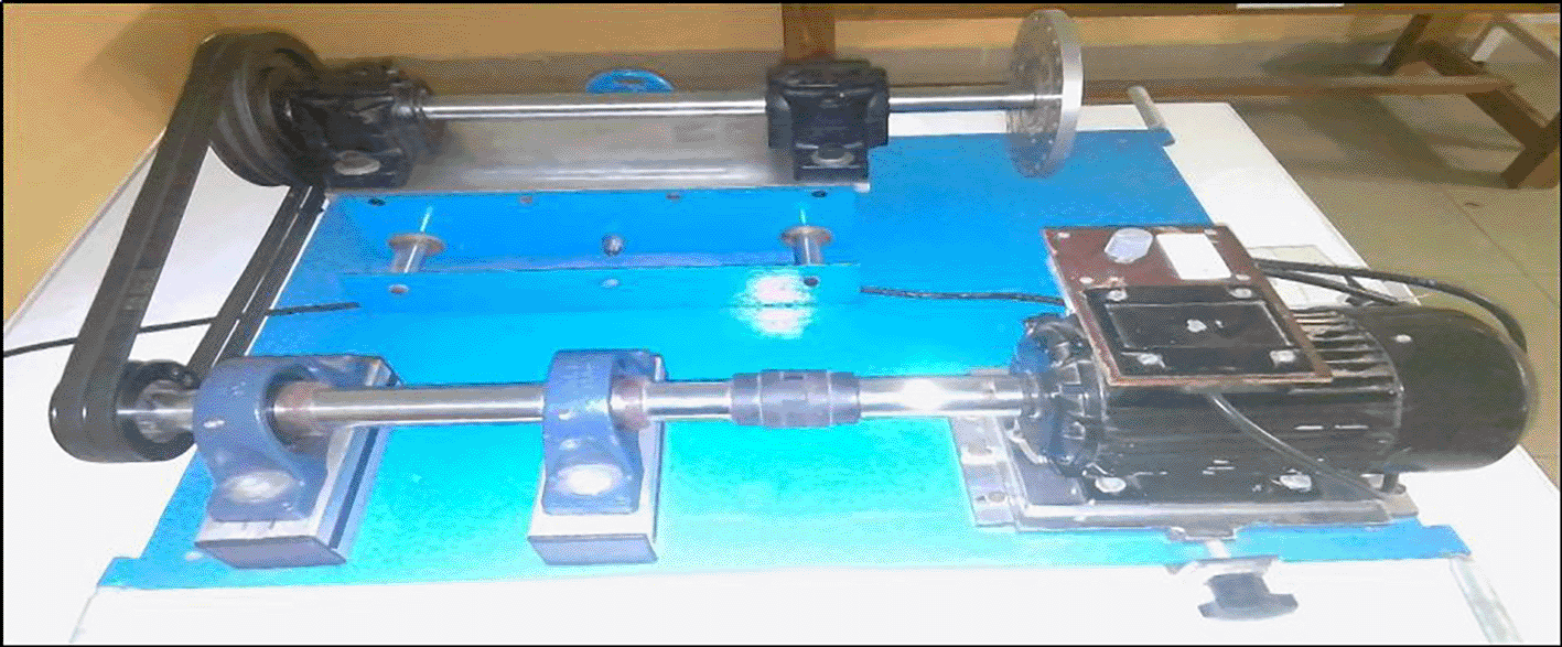
The dynamic acceleration of the system was measured through magnetic base accelerometer 353B33. An accelerometer was attached to the bearing housing in the radial direction. The probe of the accelerometer was further connected to the FFT analyzer to obtain frequency-form data. Finally, the FFT analyzer (OROS-3 series, 4 channel type) was connected to a personal computer with Noise-Vibration Gate (NV-Gate) software.

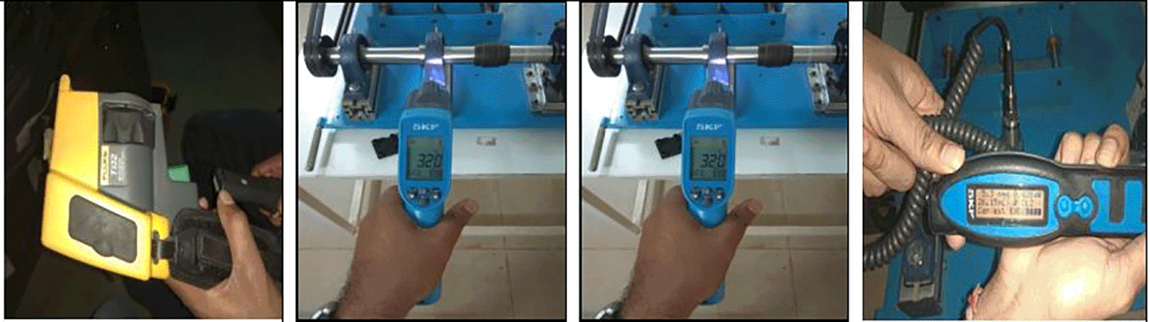
The thermal response of the test bearing was measured using a Fluke thermal imaging camera (Ti32) and an SKF Infrared digital noncontact thermometer (TKTL-30). The sound level was recorded using a Metrix digital sound level meter (SL-4005) by keeping it near the test bearing. Here, the SKF Machine Condition Advisor (MCA) was used to measure the velocity and envelope acceleration and to obtain knowledge of the test bearing condition at different points in time. The magnetic base accelerometer of the MCA was attached over the test bearing housing in the radial direction to accumulate data on the health of the bearing is shown in Figure 2.

Figure 2. Fluke Thermal imaging camera, SKF Infrared thermometer, Metrix Digital sound level meter and SKF Machine condition advisor.

3. Experiments

This section describes the experimental procedure and provides justification for the selected fault sizes and data acquisition parameters.

Before starting the experiment, adequate and specified lubricants and grease were provided to all bearings present in the setup. Experiments were performed at a constant speed of 1510 rpm for the induction motor, and at a frequency of 50 Hz. Sampling frequencies of 400, 1000, and 2000 Hz were selected to collect the vibration data for the frequency domain analysis, and a sampling time of 60 s was selected for the time-domain analysis. The bearing temperature, sound value, and condition through the MCA were recorded for 30 s after a saturation time of 15 min from the start of the setup from rest. The baseline condition of the test bearing and setup was first established by collecting the data of the fresh bearing. Subsequently, the data were collected for different faulty bearings, misalignments, unbalance, and a combination of faults. The thermal imaging camera and infrared thermometer distance and angle were kept constant from the target area to ensure that the temperature trend changed only because of the fault in the bearing and shaft. Similarly, sound measurements were performed by keeping the sound level meter at a consistent distance from the fresh bearing and the faulty bearing.

The fault sizes of 500 μm, 1000 μm, and 1500 μm were selected to represent early-stage, moderate, and severe bearing defects, respectively, as commonly reported in bearing fault diagnosis literature. Sampling frequencies of 400 Hz, 1000 Hz, and 2000 Hz were chosen to adequately capture bearing characteristic frequencies while remaining within the operational bandwidth of the accelerometer and FFT analyzer. A sampling duration of 60 s ensured sufficient signal stability for time–frequency and machine learning analysis. These parameter selections provide a balance between diagnostic accuracy and computational efficiency, making the approach suitable for practical condition monitoring applications.

To validate the proposed technique, a set of experiments was conducted: first, with a fresh bearing and then with faulty bearings (single and combination of faults in different bearing components) and shaft defects. Hence, in this study, 28 faults were considered for the experimentation process. These bearing faults were produced by an Electrical Discharge Machine (EDM).

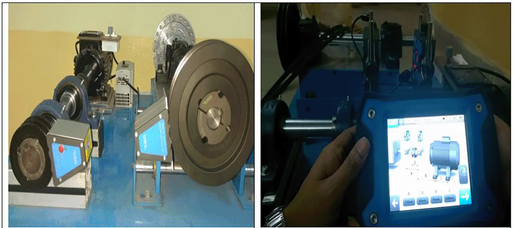
Figure 3. Alignment of pulley and shaft using SKF Laser alignment system and Belt alignment tool.

First, before starting the experiment, the entire setup was aligned using the SKF Laser alignment system (TKSA 41) and SKF Belt alignment tool (TKBA 40) shown in Figure 3 to eliminate any preexisting shaft and pulley misalignment. This is because the misalignment in the shaft has its own vibration pattern, which results in inaccurate vibration values for fresh bearings.

A magnetic base accelerometer was mounted over the housing of the test bearings to collect the vibration data. The vibration signals were processed using MATLAB wavelet design and analysis software. Different shaft and bearing faults were classified using the ANN-Pattern Recognition tool and SVM.

The test bearing has the following characteristic frequency²³:

Ball pass frequency of the outer race,BPFO=(N60×n2)×(1−dDcosθ)=90.6Hz

Ball pass frequency of the inner race,BPFI=(N60×n2)×(1+dDcosθ)=135.9Hz

Ball spin frequency,BSF=N60×Dd×(1−(dDcosθ)2)=108.72Hz

Fundamental train frequency,FTF=(N60×12)×(1−dDcosθ)=10.066Hz

4. Results and discussion

4.1 Wavelet analysis of the vibration data by complex Morlet wavelet

A wavelet is a function that is confined to time and frequency, generally with a zero mean. Using the wavelet function, a signal can be decomposed into location and frequency. Information regarding the time and frequency locations of a signal is generally present in a wavelet.

The Morlet wavelet is a Fourier exponential (complex) function with a Gaussian envelope. Hence, it ensures the signal localization. It is generally implemented for the time-frequency technique, where the Gaussian tapers a complex sine wave. The signal in the time series is then convolved with the complex Morlet wavelet. A complex-valued signal is generated as an outcome of the intricacy in between the time-series signal and complex Morlet wavelet. Hence, at each time period, the instantaneous phase and power factor of the signal can be extracted. In the wavelet convolution process, at all time points, the signal is equated with a Gaussian windowed sine wave template. This results in a time-series signal that is similar to the original signal and wavelet.²⁴

The combination of a complex sine wave and a Gaussian window is known as a complex Morlet wavelet “w.”²⁵:

w=e2iπfte−t22σ2

where “i” stands for imaginary operator (i = −1 ), “f” stands for frequency in Hz, “t” stands for time in seconds and “ σ" represents the width of the Gaussian, which is described as

σ=n2πf

The factor that states the time-frequency precision trade-off is “n”, which is often referred to as the number of cycles.

4.1.1 Application of complex Morlet wavelet on the fault detection of deep groove ball bearing

Fresh bearing

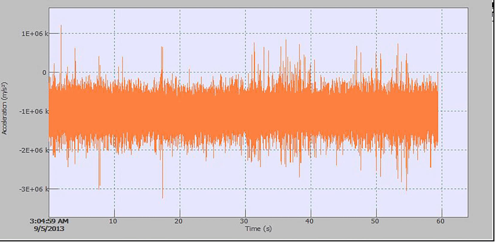
Figure 4. Time domain vibration signal of fresh deep groove ball bearing.

The Figure 4 represents the time form vibration signal of the fresh test bearing. The vibration signal of the time form clearly indicates the impact of periodic nature. The maximum amplitude of time from the vibration signal does not indicate any substantial deviations in the pattern. The frequency factor of the vibration signal did not change considerably.

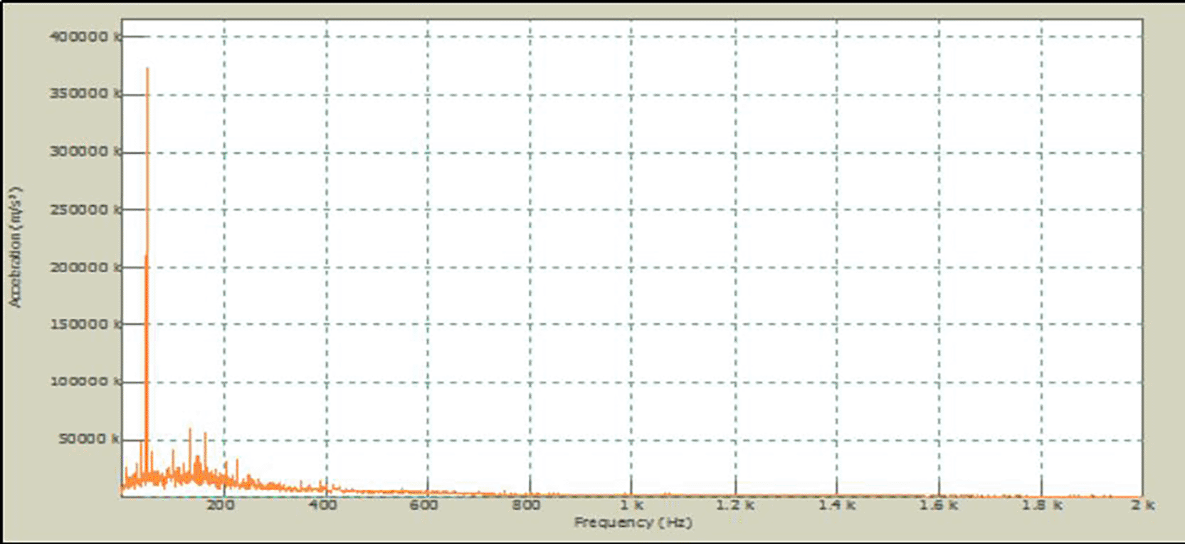
Figure 5. Frequency domain vibration signal of fresh deep groove ball bearing.

The frequency-domain vibration signal generated from the fresh test bearing is illustrated in Figure 5. According to this graph, the signal has corresponding harmonics, and there is no distinguishing error frequency factor.

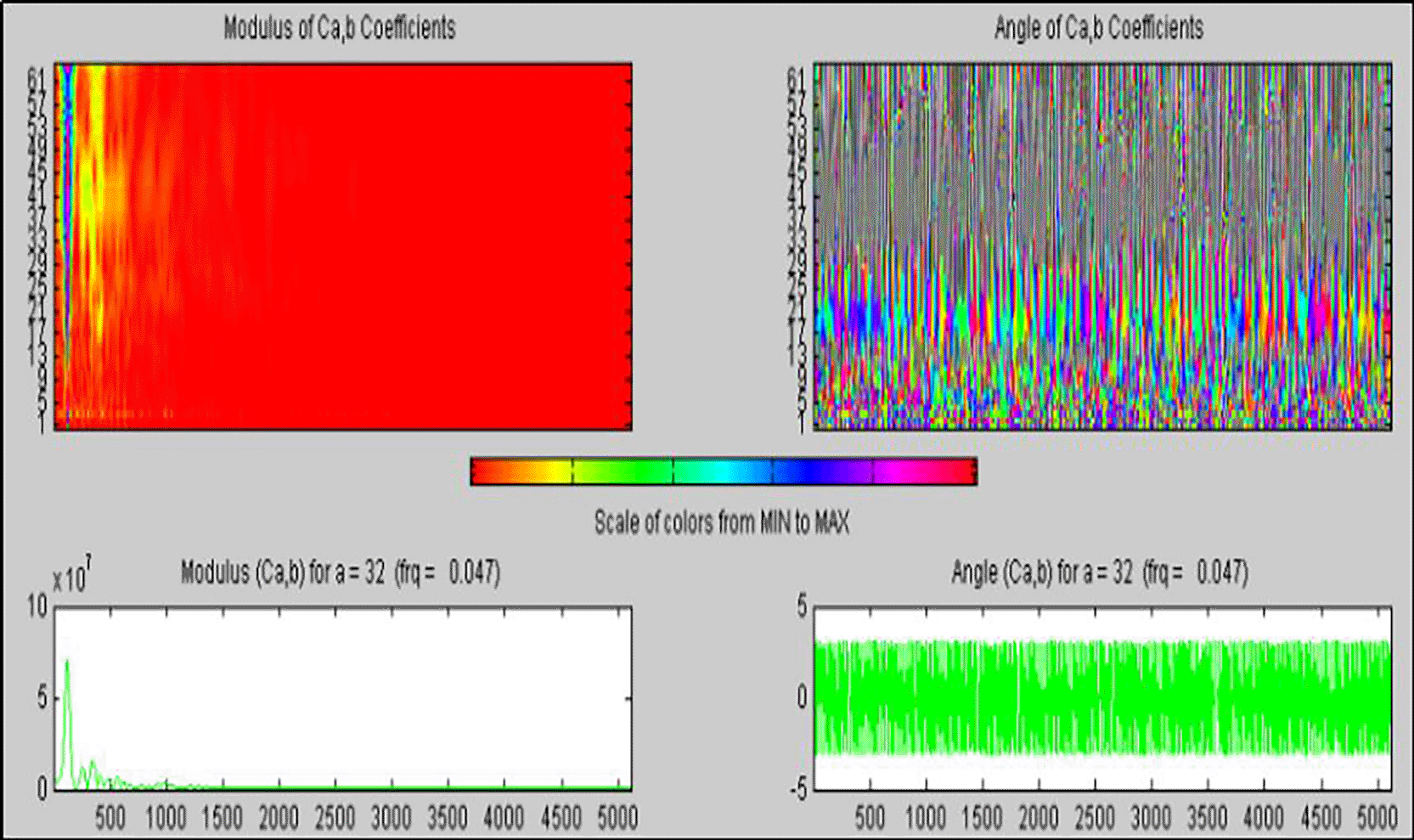
The data in Figure 5 were taken as the input parameters to generate the phase and amplitude maps of the Complex Morlet Wavelet in the MATLAB wavelet analysis tool. The results are shown in Figure 6. The maps in Figure 6 that, the vibration signature ensures that there are no identified fault features.

Figure 6. The amplitude and phase maps of the Morlet wavelet for the vibration signal with fresh bearing.

Ball, inner race and outer race combination fault of 500 micron

The Figure 7 indicates the vibration signal in the time form corresponding to the combination fault of the ball and inner and outer races of magnitude 500 μm. The vibration signal of the time form indicates an impression of the periodic pattern. The time from the vibration signal indicates substantial fluctuations in the ultimate amplitude.

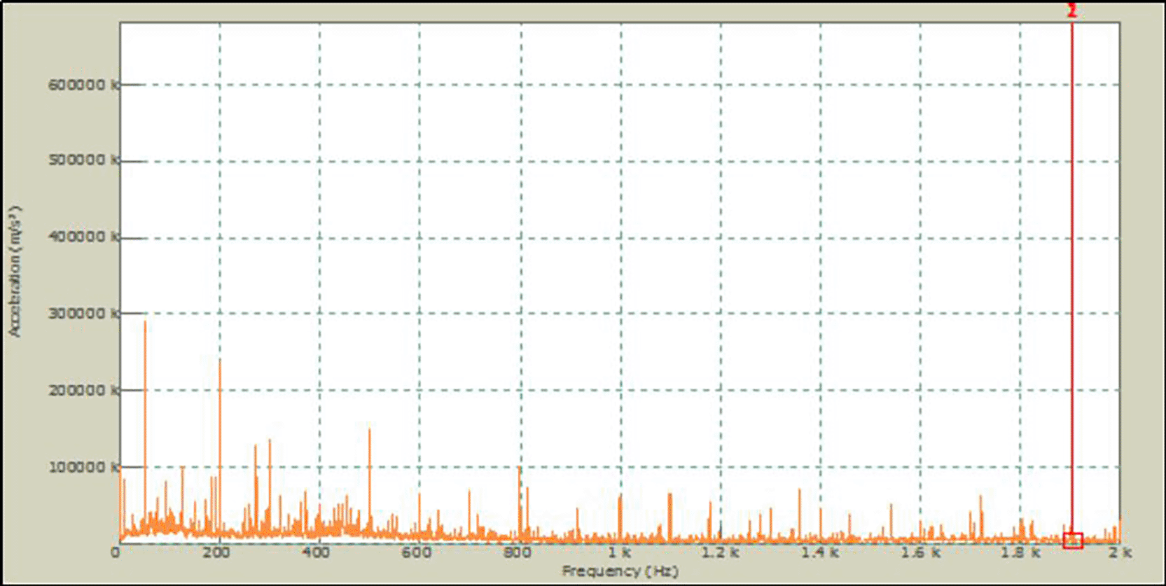
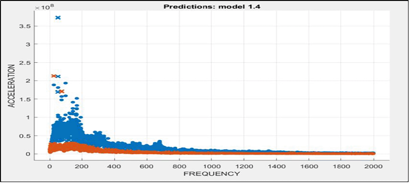
Figure 7. Time domain vibration signal of inner race, ball and outer race combination fault of 500 micron.

The Figure 8 indicates the vibration signal in frequency form corresponding to the combination fault generated in all the components of the bearing with a magnitude of 500 μm. There were no significant characteristic fault frequency factors near the theoretical characteristic frequency of the bearing components. This signifies the limitation of the frequency domain analysis to effectively indicate the fault frequency factor of the combination fault generated in all components of the test bearing.

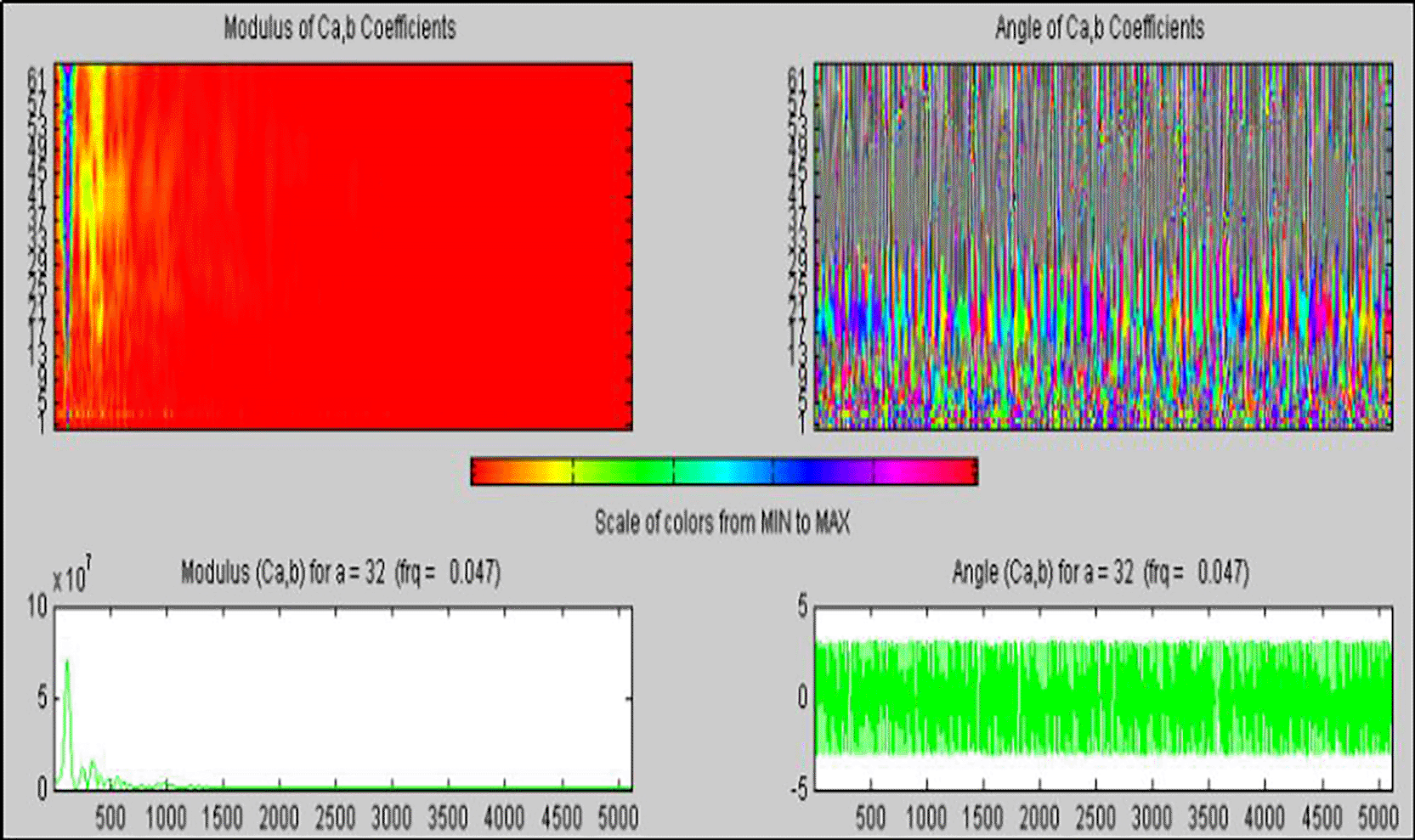
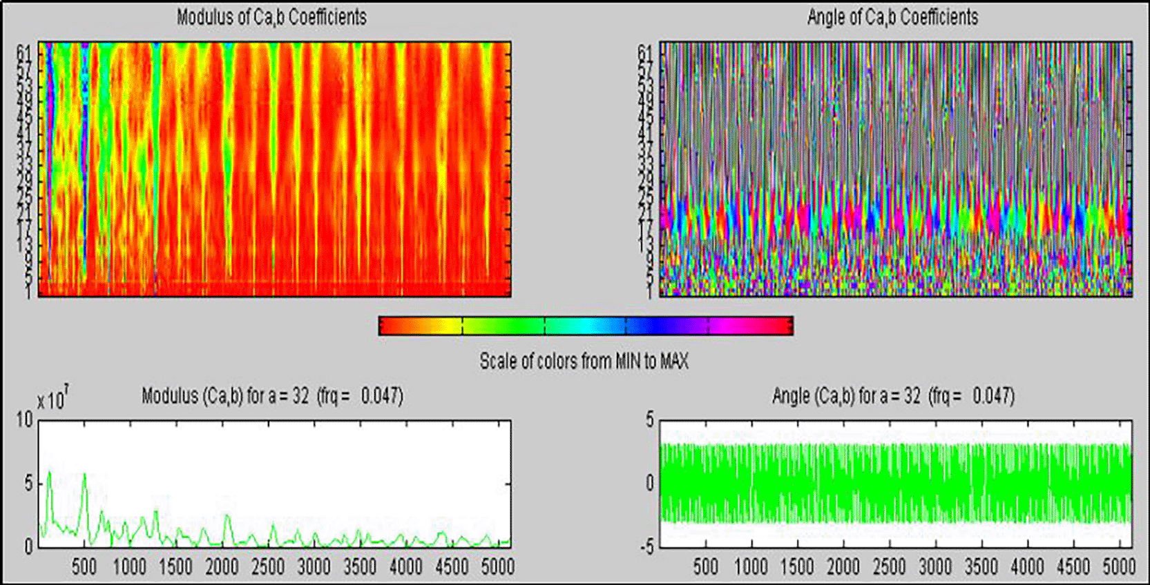
Figure 8. Frequency domain vibration signal of inner race, ball and outer race combination fault of 500 micron.

The Figure 9 noticeably specifies amplitude and phase maps of the Morlet wavelet with a combination fault in the test bearing. The energy level corresponds to the rapid increase in vibration owing to the existence of a combination fault. The transient vibration from the combined bearing faults is clearly indicated by higher-order harmonics and characteristic defect frequencies. The transient vibrations show a monotonous pattern, which is a sign of repetitive characteristic faults, and the excited intrinsic mode of the test bearing shows a chain of transitory vibrations at the resonant frequencies, which is the effect of the generated defect. The Morlet wavelet phase map was considerably clearer than the amplitude map. In addition, the phase map showed a more profound correlation with the amplitude map.

Figure 9. The amplitude and phase map of combination fault of 500 micron.

4.2 Artificial Neural Network (ANN)

An ANN is analogous to the nervous system of the human body, whose function is to process information. Vital applications, such as pattern recognition or classification of specific data, can be performed using an ANN through a learning procedure.

It generally comprises two periods: the learning or training stage, and the testing or simulation stage. The training period initializes the weights and biases of the ANN to any random standard. The learning and momentum rates are the training parameters that are selected accordingly. Additionally, appropriate definitions of the training termination criteria, such as the maximum number of epochs and training parameter limits, were selected. The learning stage in the ANN framework can be observed as a complication of updating the network building and linking weights, such that a network can proficiently accomplish a definite job. During this process, the artificial neural network generally studies the linking weights from the presented training configurations. The performance of the neural network increases when the weights are updated in steps over time. The training period stopped in the ANN once the training termination requirements were fulfilled. The neural network was trained with the chosen data, and the model was again tested with the leftover data. Network performance is evaluated by comparing the desired output with the output of the neural network.^26,27

ANN can be used as a potential tool for classifying and predicting bearing faults. In the ANN segment, the process of pattern recognition is implemented as a significant classifier to categorize different faults in the shaft-bearing system, owing to its characteristics of following a definite pattern. Here, “nptool” is used to train the data by importing the input and output parameters to the MATLAB workspace. In this method, a conjugate gradient backpropagation training algorithm is used to train the neural network. For repetitive training of the network, the assigned weights were modified frequently, and multiple iterations were performed to achieve the best classification result.

The major goal of this study is to differentiate between fresh and faulty bearings; hence, in the pattern recognition tool, a binary classification scheme was used. Where, ‘1 0 0’ was used for fresh bearing, ‘0 1 0’ for inner race fault bearing and ‘0 0 1’ was used to indicate the outer race fault bearing. Here, a mean square error (MSE) of 10⁻³, a least gradient of 10⁻¹⁰ and extreme number of epochs of 1000 were implemented. The training progression was terminated automatically whenever the above-mentioned circumstances were achieved. The initial biases and weights of the ANN were set arbitrarily.²⁸

Ball and inner race combination fault of 1000 micron

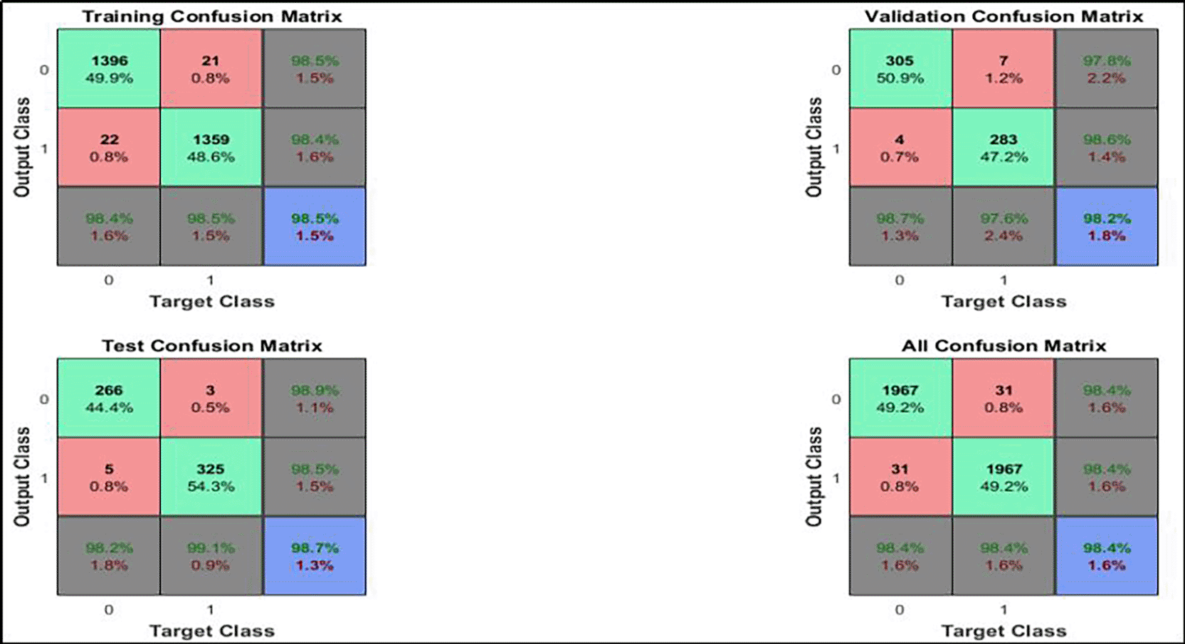
Using acceleration and frequency value of the combined fault of 1000 micron in the ball and inner race of the test bearing as the input parameter the neural network and the bearing condition as the target value, the best performance of the ANN classification technique was found to be 98.4%.

The Figure 10 depicts the confusion matrix of the ball and inner race fault of 1000 microns using ANN. Using the features from the vibration signals, the proposed pattern recognition technique of ANN shows the best performance and a superior level of exactness in classifying the faults of deep groove ball bearings effectively.

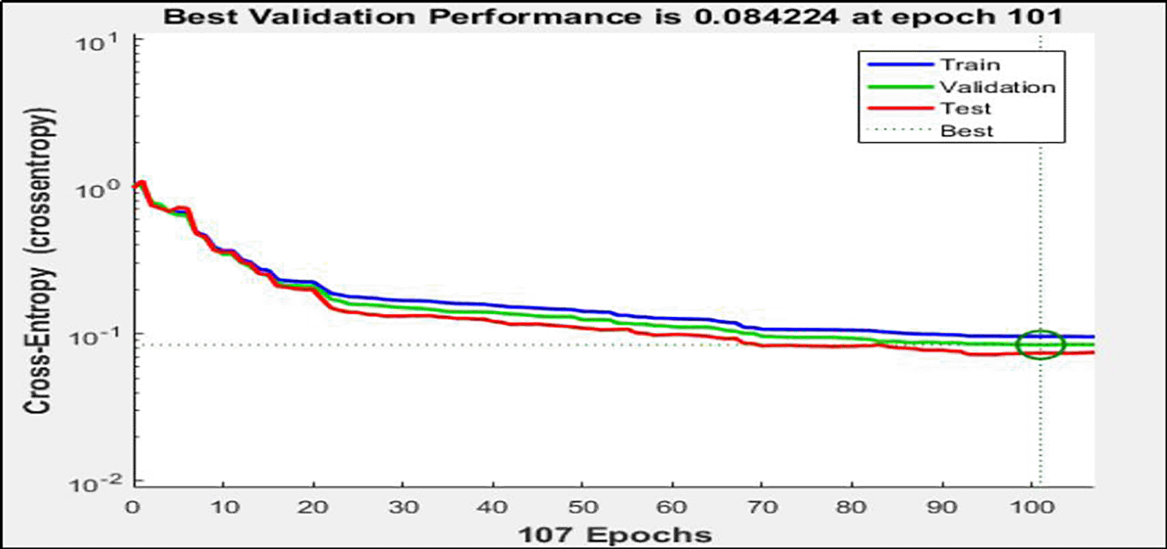
Figure 10. Confusion matrix of combination fault and fresh bearing.

The Figure 11 specifies the best validation performance curve for a combination fault of 1000 μm in the ball and inner race of the test bearings. The best classification result of 98.4% was achieved at epoch 101, and the corresponding validation performance was 0.084224. Because this value is less than 0.5, it is within the acceptable level.

Figure 11. Best validation performance graph of combination fault and fresh bearing.

From the Table 1 this indicates that the implementation of an ANN-based pattern recognition technique can effectively classify different bearing faults.

Table 1. Classification accuracy percentage and best validation performance of ANN.Type of fault Fault magnitudeANN classification accuracyTrain-Test-Validation dataBest performance value Epoch Ball fault500 micron72.9%70-15-150.1048718 Inner race fault500 micron75%80-10-100.1406219 Outer race fault500 micron75%80-10-100.2728414 Inner race fault1000 micron90.4%70-15-150.22935132 Outer race fault1000 micron88.9%80-10-100.31702108 Ball fault1000 micron93.8%60-20-200.19371108 Inner and outer race combination fault1000 micron98.6%60-20-200.05492173 Ball and inner race fault1000 micron98.4%70-15-150.084224101 Ball and outer race fault1000 micron100%70-15-150.04920459 MisalignmentMedium95.7%70-15-150.2173542 UnbalanceHigh70.5%70-15-150.6396254

4.3 Support Vector Machine (SVM)

SVM uses a hyperplane to distinguish between the two types of data. In this process, the SVM generates a separation line between the two classes of data. During data analysis, support vector machines generally create a hyperplane between datasets of two different classes. Subsequently, to solve this problem, SVM generates a hyperplane. The points adjacent to the margin are called the support vectors of the machine algorithms. The boundary region between the margins was represented by the midline. The hyperplane divides the plane into two different fragments in the 2-D region, where each class of data lies on either side. The fundamental idea lies in this method to segregate data in two different classes described by a support vector by means of a hyperplane.^29,30

The hyperplane equation of SVM is given as,³¹

Here, the “w” vector express the border, “b” is a bias or in other words is a scalar threshold and “x” is the input vector.

The support vectors are placed at the margins in terms of two different classes expressed as³¹:

The terminology “Fresh” and “Fault” was used to classify the different bearing conditions. For the classification of data, a fivefold cross-validation method was implemented, as it protects the information from overfitting. Different SVM methods were used to train the model. A superior level of accuracy was achieved by manually selecting the kernel function and scale.

In this study, the performance of the SVM classifier was determined by plotting a confusion matrix. The positive or negative rate of the trained SVM model was determined by plotting the receiver operating characteristic (ROC) curve. The overall performance of the SVM classifier was evaluated using the area under the curve (AUC).

Combination fault of 1000 micron in the ball and inner race of the test bearing

The features abstracted from the vibration signal were used as the input parameters for the SVM classifier. The Figure 12 indicates the scatter plot of the fresh bearing and ball-inner race combination fault of 1000 μm. Here, the scatter plot clearly differentiates the two bearing conditions by two different color indications, where the fresh bearing parameters are indicated by red color marks, and the ball-inner race combination faults are indicated by blue color marks.

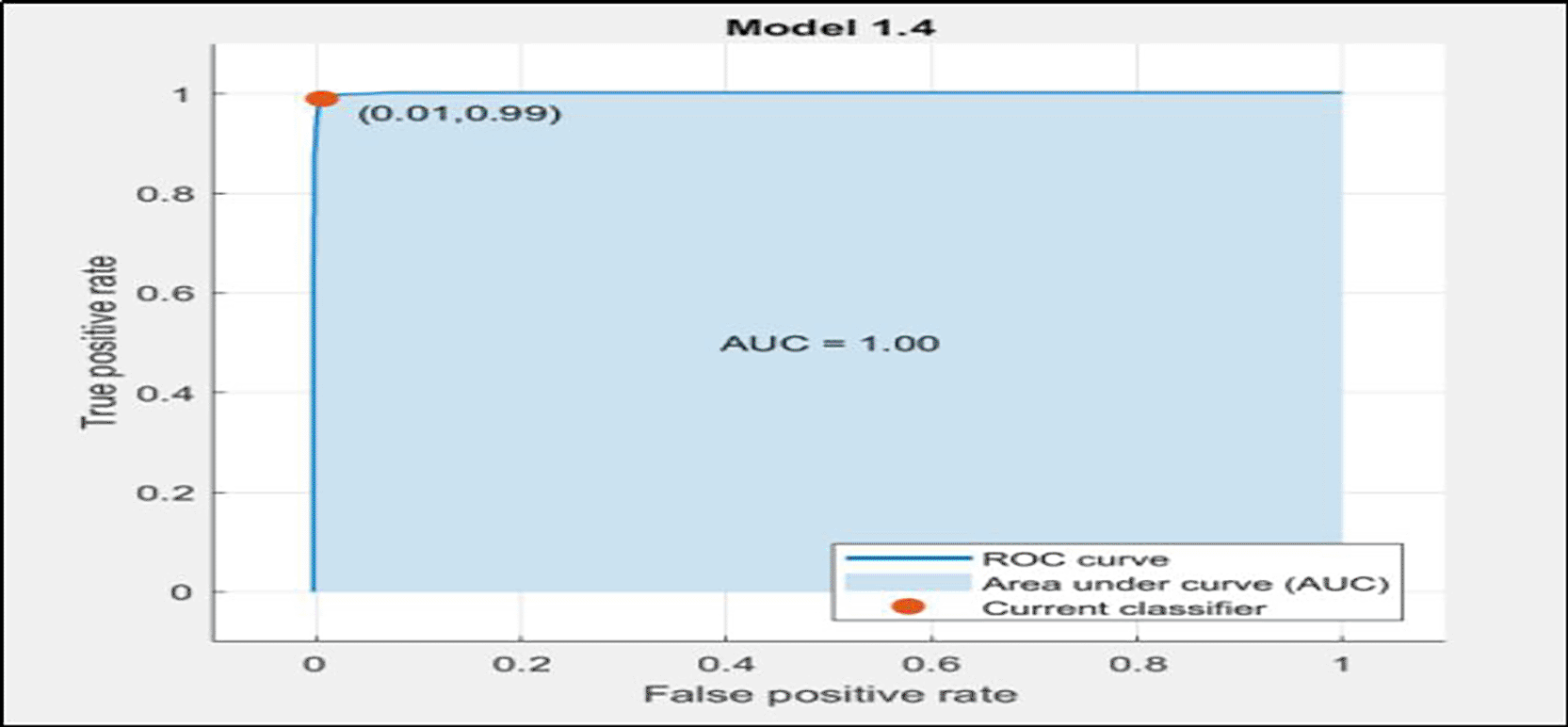
Figure 12. Scatter plot of fresh bearing and ball-inner race fault of 1000 micron.

Figure 13. ROC curve of fresh bearing and ball-inner race fault of 1000 micron.

The ROC curve shown above in Figure 13 specifies that the proposed SVM classifier classifies the ball and inner race combination fault of 1000 μm more accurately, as the true positive rate of the classifier was found to be 99% and the false positive rate was only 1%. The overall accuracy of the classifier was 100%, as indicated by the area under the ROC curve of 1.00.

Finally, different shaft and bearing faults were taken as the input parameters for the SVM classifier, and the corresponding classification accuracy was represented in tabular form as follows.

Table 2. Classification accuracy percentage and best validation performance of SVM.Type of fault Fault magnitudeSVM classification accuracyTrain-Test-Validation dataBest performance value Iterations Ball fault500 micron78.2%70-15-150.0913462 Inner race fault500 micron80.6%80-10-100.1182774 Outer race fault500 micron79.8%80-10-100.1946269 Inner race fault1000 micron92.7%70-15-150.18241118 Outer race fault1000 micron91.3%80-10-100.25638103 Ball fault1000 micron95.1%60-20-200.1719697 Inner and outer race combination fault1000 micron99.1%60-20-200.0438585 Ball and inner race fault1000 micron98.9%70-15-150.0612794 Ball and outer race fault1000 micron99.6%70-15-150.0389471 MisalignmentMedium96.8%70-15-150.1984258 UnbalanceHigh73.4%70-15-150.5812666

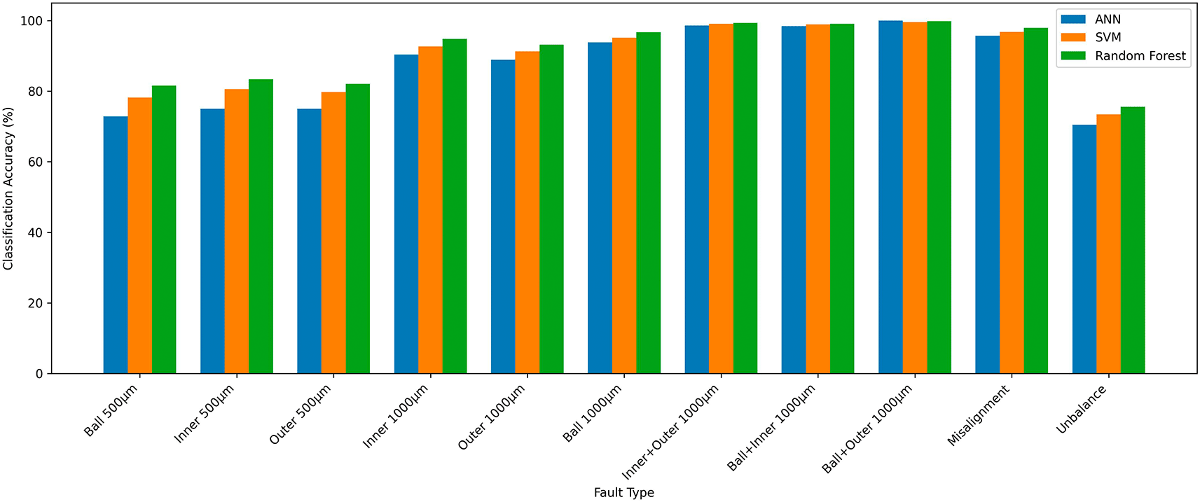
The inclusion of the Random Forest classifier further improved the fault diagnosis performance. As shown in Figure 14, Random Forest achieved the highest classification accuracy for most fault categories, particularly for low-severity faults (500 μm), where it outperformed both ANN and SVM. For severe faults (1000 μm) and combined fault conditions, all three classifiers exhibited excellent performance with accuracies approaching 100%; however, Random Forest maintained a slight advantage in most cases. The results indicate that ensemble learning effectively captures complex fault patterns and provides better generalization than individual classifiers. Among the evaluated methods, Random Forest demonstrated the most consistent performance across all fault categories, followed by SVM and ANN. Nevertheless, all three classifiers showed relatively lower accuracy for the unbalance condition, suggesting the need for more discriminative features for this fault type.

Figure 14. Classification accuracy comparison of ANN, SVM, and Random Forest for various bearing faults and machine conditions.

4.4 Other techniques

4.4.1 Bearing temperature analysis by thermal imaging camera

In this study, first, the temperature reading and thermal behavior of the fresh bearing under operation conditions were determined by a non-contact laser thermometer and a Fluke Thermal imaging camera. Subsequently, the same process is repeated for different faulty bearings by mounting them in the test rig. The mutual effects of temperature and bearing conditions were analyzed accordingly. The temperature rise difference between fresh and faulty bearings was then proposed to monitor the bearing condition. Different bearing and shaft conditions, that is, fresh (reference), ball fault, inner race fault, outer race fault, unbalance, misalignment, and combined faults, are used to observe the performance of the existing system.

Fresh bearing

To measure the temperature of the bearing, a thermal imaging camera was focused on the bearing housing at a distance of one meter. An image of the specified location was captured using a thermal-imaging camera. Subsequently, the captured images were analyzed using Smart View 4.3 software. Smart View software was used to transfer the image from the thermal imaging camera to the computer system. From the captured image, using the Smart View software, the 3D-Infrared fusion image and histogram graph were plotted. These plots can be utilized as powerful tools for estimating the condition of rolling element bearings. First, an image of the fresh bearing in the operating condition was captured using a thermal imaging camera. Further, the image was processed using Smart View software. The corresponding thermal image, 3D-Infrared fusion image, and histogram graph are shown in Figure 15.

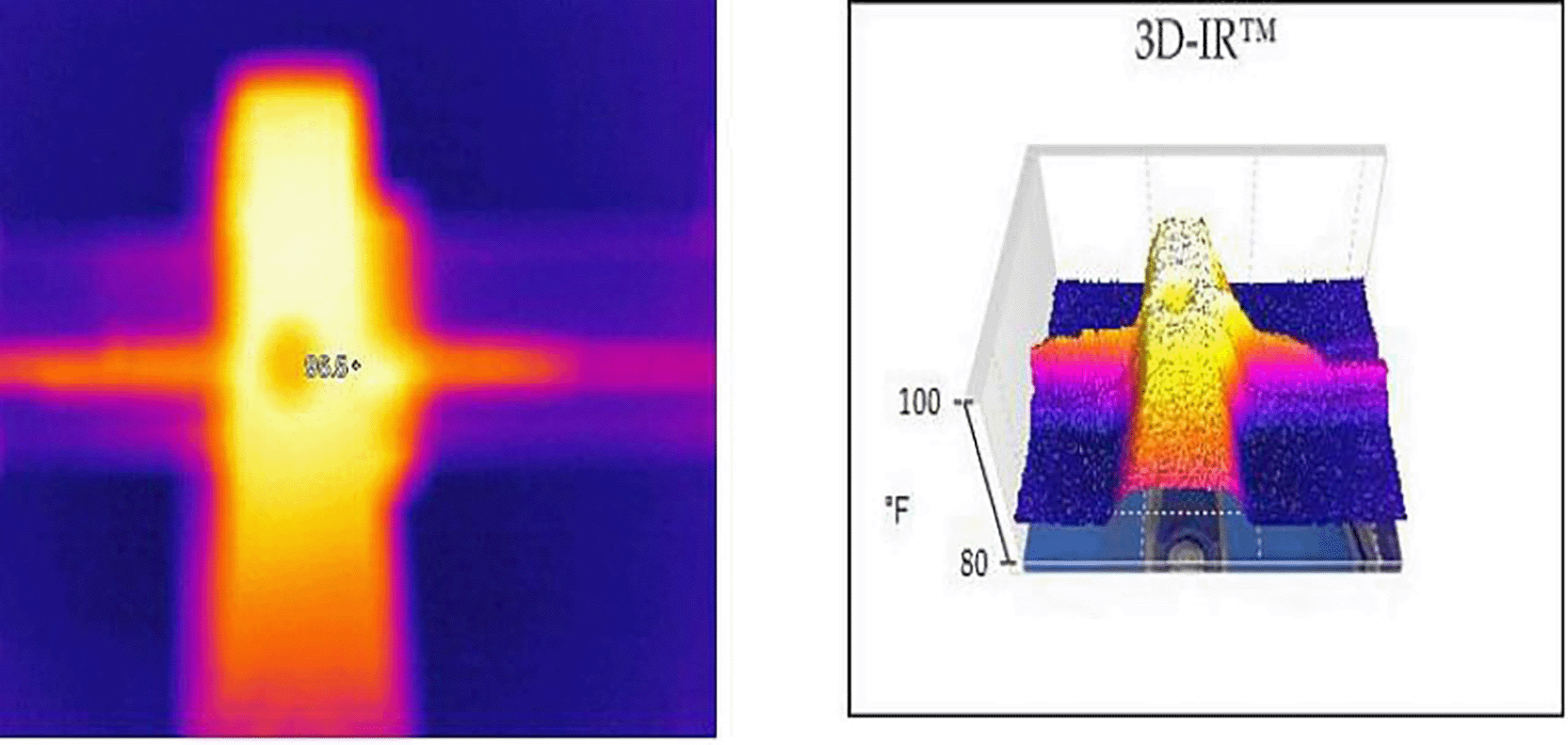
Figure 15. Thermal image and 3D-Infrared fusion image of fresh bearing.

The thermal image of the fresh bearing indicates that at the specified location the temperature was found to be 96.5°F. The pattern of the temperature distribution over the bearing housing is represented by different color combinations of the specified intensity. The 3D- Infrared fusion image also indicates the variation in temperature throughout the specified location of the shaft bearing system using a 3D image. It also indicates the fluctuation of the pattern between 80°F and 100°F.

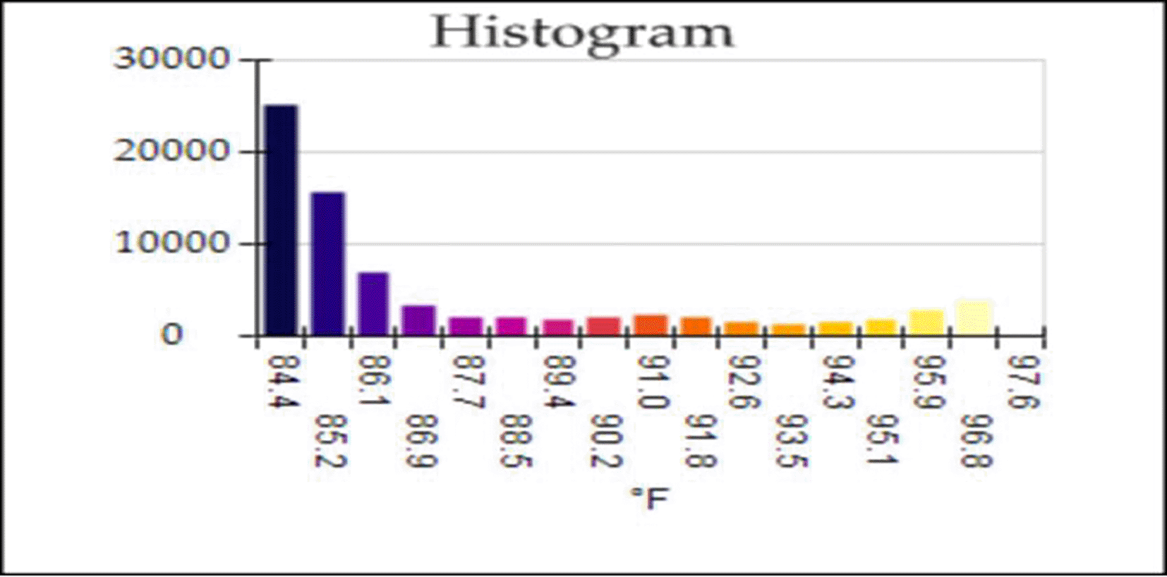
The histogram shown in Figure 16 of the fresh bearing represents the rate of recurrence at the specified temperature. The histogram graph is plotted by considering the image pixels along the vertical axis and the temperature (in °F) along the horizontal axis. Equal-sized bins were used to divide the image’s temperature range. The height of the graph indicates the number of pixels with temperatures that fall within the range of the bin. The histogram represents the temperature variation between 84.4°F 97.6°F.

Figure 16. Thermal histogram graph of fresh bearing.

500 micron outer race fault

After introducing a fault of 500 μm in the outer race of the bearing, the complete shaft-bearing system was again viewed under the thermal imaging camera. The thermal image of a 500 micron outer race fault bearing shown in Figure 17 indicates that at the specified location, the temperature was found to be 110.9°F. The pattern of the temperature distribution over the bearing housing is represented by different color combinations of the specified intensity. The 3D- Infrared fusion image also indicates the variation in temperature throughout the specified location of the shaft bearing system using a 3D image. It also indicates the fluctuation of the pattern between 80°F and 120°F. This elevation in temperature level compared to the previous case of fresh bearing is a clear indication of a fault in the bearing.

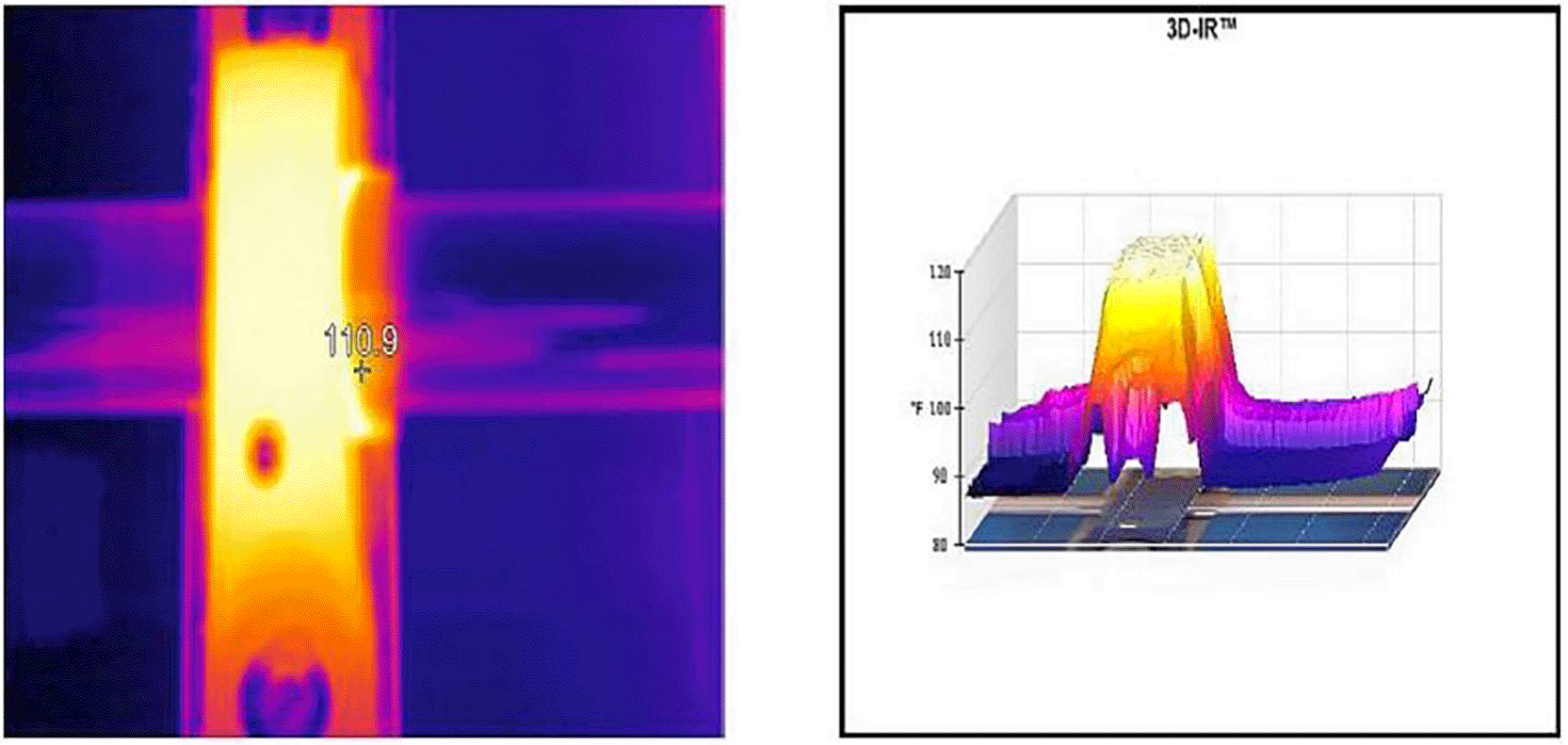
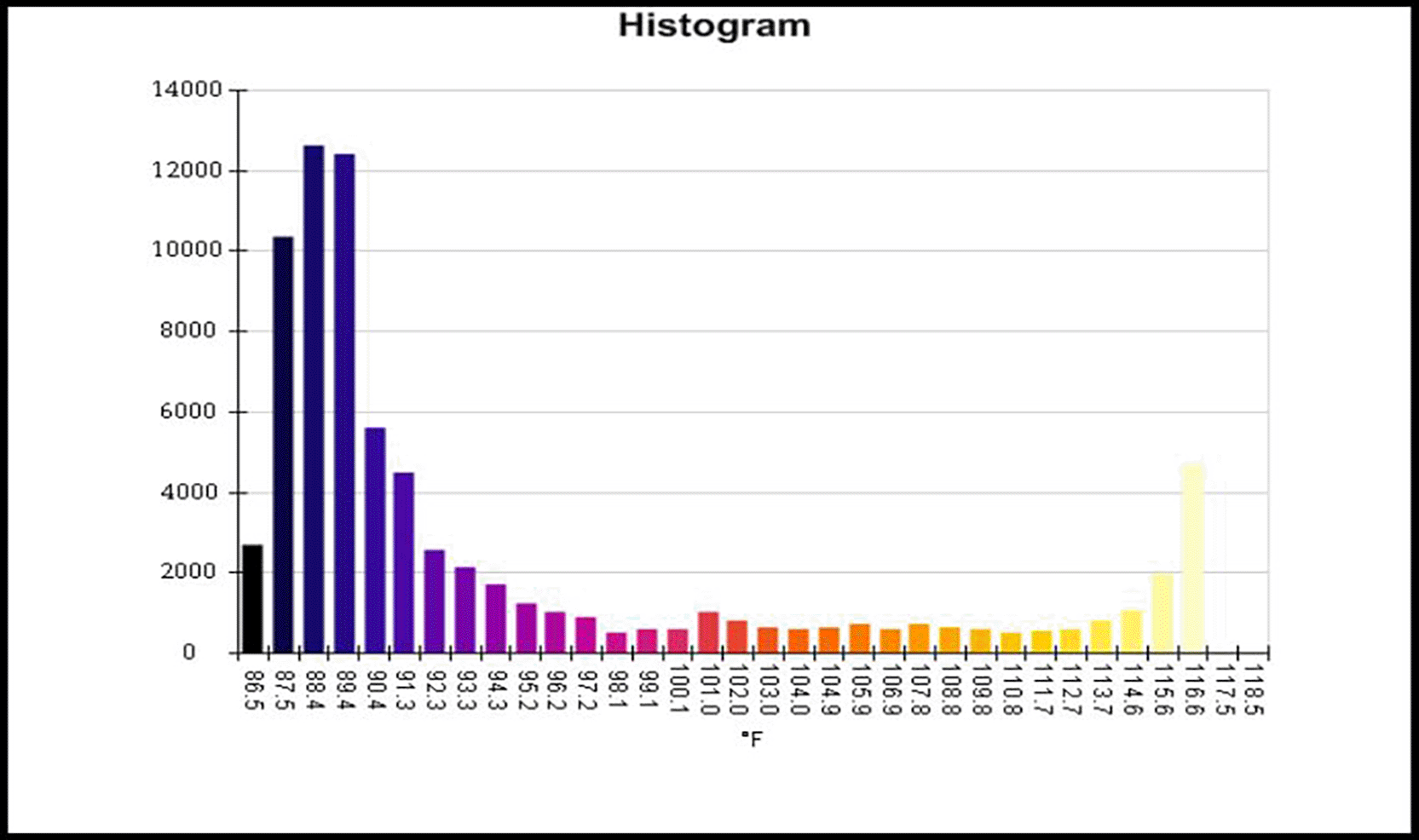
Figure 17. Thermal image and 3D-Infrared fusion image of 500 micron outer race fault bearing.

The histogram graph shown in Figure 18 of the outer race of a 500 micron fault bearing represents the rate of recurrence of the specified temperature with respect to the image pixel. The height of the graph indicates the number of pixels with temperatures that fall within the range of the bin. The histogram graph represents the temperature variation in between 86.5°F to 118.5°F. It also indicates that the temperature of 116.5°F is present over an approximately 5000 pixel range, which is higher than the case of fresh bearing. Hence, the histogram of the thermal imaging camera can be utilized to supervise the condition of a rolling element bearing.

Figure 18. Thermal histogram graph of outer race of 500 micron fault bearing.

4.4.2 Bearing condition monitoring by Machine condition Advisor

Here, the SKF Machine Condition Advisor (CMAS100-SL) was used to measure the velocity and enveloped acceleration, and to obtain knowledge of the bearing condition at different times. The device shows the total velocity vibration value, which computes vibration signals from the machine and equates those readings with the pre-programmed guidelines of the International Organization for Standardization (ISO). The device shows the prompt of an “ALERT” or “DANGER” whenever the measured values cross the guidelines. The device also measure an “ENVELOPED ACCELERATION” and compares with standard guidelines of bearing vibration to validate conventionality or specify possible bearing damage. It also indicates the uncharacteristic heat by measuring the temperature using an infrared sensor. The device could be connected externally with a standard 100 Mv/g constant current acceleration.

The SKF CMAS100-SL machine condition advisor measures the velocity range 0,7-65,0 mm/s (Root Mean Square) or 0.04-3.60 in. /s (equivalent peak), which meets ISO 10816-3, The frequency range of 10–1000 Hz, which meets ISO2954. The enveloped acceleration can be measured within the range of 0,2-50,0 (gE), while the frequency ranges from to 500-10000 Hz (Band 3). The device can measure the temperature with an accuracy of 2°C°F (Infrared temperature) ranging between -20 to 200°C (-5 to 390°F) from the short distance range, maximum 4 inches or 10 cm from the target. The device is IP54 rated and can be used in working temperature range of -10 to 60°C (15 to 140°F) whereas in charging mode it can be operated in 0 to 40°C (30 to105°F) range.

This advisor offers a way to assess the health of the machine in accordance with ISO 10816-3 and to assess the bearings in accordance with universal standards created from a statistical study of prevailing databases.³²

New bearing

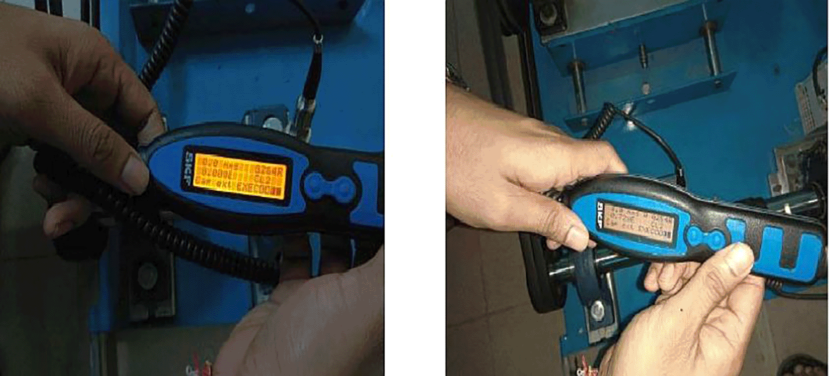
An accelerometer with a magnetic base is mounted on the test bearing housing shown in Figure 19. First, a fresh bearing was considered for the analysis. The accelerometer probe is connected to a machine condition advisor. Readings were taken 15 min after running the setup. The Machine condition advisor showed readings of 4 mm/s (velocity), 0.72gE (envelope acceleration), A (alarm display), CL2 (envelope acceleration class), G2, and 4R (ISO Machine group). Here, the envelope acceleration of 0.72gE represents that the bearing is in good condition. The alarm display reading (A) represents the healthy condition of the bearing. The envelope acceleration class CL2 indicates that the bearing bore diameter is between 50 and 300 mm. In addition, this indicates that the shaft speed was between 500 and 1800 rpm. The ISO machine groups G2 and 4R show that the setup is an electrically driven machine with shaft heights between 160 mm and 315 mm. This also indicates that these machines are equipped with rolling-element bearings.

Figure 19. New bearing conditions monitoring by SKF Machine Condition Adviser.

1500 micron ball fault and misalignment-high

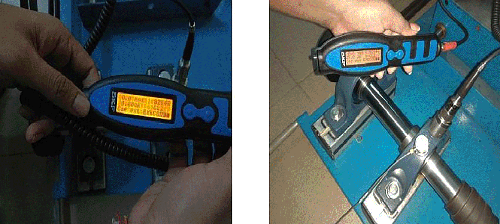
An accelerometer with a magnetic base was mounted over the housing of a 1500 μm ball fault bearing connected to a shaft of high-level misalignment shown in Figure 20. The accelerometer probe is connected to a machine condition advisor. Readings were taken 15 min after running the setup. The Machine condition advisor showed readings of 8.8 mm/sec (velocity), 25.06gE (envelope acceleration), D (alarm display), CL2 (envelope acceleration class), G2, and 4R (ISO Machine group). A velocity of 8.8 mm/sec is an indication of a fault in the bearing. Here, an envelope acceleration of 25.06gE represents that the bearing has a severe fault. The alarm display reading (D) also indicates that the bearing is in the “Danger” condition, and it is the time to change the bearing. The envelope acceleration class CL2 indicates that the bearing bore diameter is between 50 and 300 mm. In addition, this indicates that the shaft speed was between 500 and 1800 rpm. The ISO machine groups G2 and 4R show that the setup is an electrically driven machine with shaft heights between 160 mm and 315 mm. This also indicates that these machines are equipped with rolling-element bearings.

Figure 20. 1500 micron ball fault bearing & high level shaft misalignment conditions monitoring by SKF Machine Condition Adviser.

The machine condition advisor clearly indicates the bearing condition using alarm types A or D. The “Envelop acceleration class” and “ISO machine group” gives the accurate information about the setup. Hence, condition monitoring of the shaft-bearing system through a machine condition advisor can be considered as a simple and cost-effective technique. The information provided by the machine condition advisor is a deciding parameter for monitoring the bearing condition.

5. Conclusion

This research presents an integrated and intelligent condition monitoring framework for deep groove ball bearings by combining Complex Morlet Wavelet (CMW) analysis, Artificial Neural Networks (ANN), Support Vector Machines (SVM), Random Forest (RF) classification, thermographic analysis, and SKF Machine Condition Advisor tools. The experimental results demonstrate that the phase and amplitude representations derived from the Complex Morlet Wavelet effectively capture transient vibration signatures associated with bearing faults under both single and combined fault conditions. These time–frequency features provide richer and more discriminative diagnostic information than conventional time- and frequency-domain analysis methods.

A comparative evaluation of ANN, SVM, and Random Forest classifiers reveals that all three machine learning models are capable of accurately identifying bearing faults; however, Random Forest consistently achieves the highest classification performance across most fault categories. The average classification accuracies obtained using ANN, SVM, and Random Forest are 87.2%, 95.271%, and 97.48%, respectively. The superior performance of Random Forest can be attributed to its ensemble learning mechanism, which enhances robustness, reduces overfitting, and improves generalization capability. While SVM demonstrates excellent performance in handling high-dimensional feature spaces and limited training samples, ANN exhibits comparatively lower accuracy, particularly for low-severity faults. The results indicate that the Random Forest classifier is the most effective approach for the proposed fault diagnosis framework.

In addition to vibration-based fault diagnosis, the integration of thermography, infrared temperature measurement, and SKF Machine Condition Advisor tools provides complementary information for validating fault severity and machine health. The combined use of vibration and thermal analysis improves diagnostic reliability and offers a practical and cost-effective solution for predictive maintenance applications.

Although the proposed framework demonstrates high diagnostic accuracy, the experimental investigations are limited to controlled laboratory conditions and constant rotational speeds. Future research will focus on extending the methodology to variable-speed and variable-load operating conditions, exploring advanced deep learning techniques for automated feature extraction, validating the framework using large-scale industrial datasets, and implementing real-time fault diagnosis through edge and embedded computing platforms for Industrial Internet of Things (IIoT)-based condition monitoring systems.

Overall, the proposed framework provides an effective and reliable solution for intelligent bearing fault diagnosis. The integration of Complex Morlet Wavelet analysis with machine learning classifiers, particularly Random Forest, demonstrates strong potential for practical deployment in predictive maintenance, machinery health monitoring, and smart manufacturing environments.

Data availability

Figshare: Conditioning monitoring data of ball bearing based on wavelet analysis model with machine learning techniques. https://doi.org/10.6084/m9.figshare.29582633.³³

This project contains the following data:

• Ballbearing Datase.csvt (This CSV file generated and analyzed during the current study.)
• Image/ (Contains JPEG images of the processed dataset and visual outputs used in the study.)

Data are available under the terms of the Creative Commons Attribution 4.0 International license (CC-BY 4.0).

Acknowledgement

The authors would like to acknowledge the SKF-KIIT Advanced Reliability Center in the School of Mechanical Engineering at KIIT Deemed to be University, Bhubaneswar, Odisha, India, where this research work was carried out.

References

1. Ying Y, Li J, Chen Z, et al.: Study on rolling bearing on-line reliability analysis based on vibration information processing. Comput. Electr. Eng. July 2018; 69: 842–851. Publisher Full Text
2. Malla C, Panigrahi I: Review of condition monitoring of rolling element bearing using vibration analysis and other techniques. Journal of Vibration Engineering & Technologies. May 2019; 7(4): 407–414. Publisher Full Text
3. Saxena M, Bannett OO, Sharma V: Bearing fault evaluation for structural health monitoring, fault detection, failure prevention and prognosis. Procedia Engineering. 2016; 144: 208–214. Publisher Full Text
4. Shin JH, Jun HB: On condition based maintenance policy. Journal of Computational Design and Engineering. April 2015; 2(2): 119–127. Publisher Full Text
5. Upadhyay RK, Kumaraswamidhas LA, Azam MS: Rolling element bearing failure analysis: A case study. Case Studies in Engineering Failure Analysis. January 2013; 1(1): 15–17. Publisher Full Text
6. Saruhan H, Sandemir S, Cicek A, et al.: Vibration analysis of rolling element bearing defects. Journal of Applied research and Technology. June 2014; 12(3): 384–395. Publisher Full Text
7. Li CJ, Li SY: Acoustic emission analysis for bearing condition monitoring. Wear. June 1995; 185(1-2): 67–74. Publisher Full Text
8. Kiral Z, Karagulle H: Vibration analysis of rolling element bearing with various defects under the action of an unbalanced force. Mech. Syst. Signal Process. November 2006; 20(8): 1967–1991. Publisher Full Text
9. Dolenc B, Boskoski P, Juricic D: Distributed bearing fault diagnosis based on vibration analysis. Mech. Syst. Signal Process. January 2016; 66-67: 521–532. Publisher Full Text
10. Mehdizadeh M, Khodabakshi F: An investigation into failure analysis of interfering part of a steam turbine journal bearing. Case Studies in Engineering Failure Analysis. October 2014; 2(2): 61–68. Publisher Full Text
11. Zhou L, Duan F, Mba D, et al.: Using frequency domain analysis techniques for diagnosis of planetary bearing defect in a CH-46E helicopter aft gearbox. Eng. Fail. Anal. October 2018; 92: 71–83. Publisher Full Text
12. Laissaoui A, Bouzouane B, Miloudi A, et al.: Perceptive analysis of bearing defects (Contribution to Vibration Monitoring). Appl. Acoust. November 2018; 140: 248–255. Publisher Full Text
13. Seera M, Wong MLD, Nandi AK: Classification of ball bearing faults using a hybrid intelligent model. Appl. Soft Comput. August 2017; 57: 427–435. Publisher Full Text
14. Rafiee J, Arvani F, Harifi A, et al.: Intelligent condition monitoring of a gearbox using artificial neural network. Mech. Syst. Signal Process. May 2007; 21: 1746–1754. Publisher Full Text
15. Nguyen P, Kang M, Kim JM, et al.: Robust condition monitoring of rolling element bearings using de-noising and envelope analysis with signal decomposition techniques. Expert Syst. Appl. December 2015; 42(22): 9024–9032. Publisher Full Text
16. Malla C, Rai A, Kaul V, et al.: Rolling element bearing fault detection based on the complex morlet wavelet transform and performance evaluation using artificial neural network and support vector machine. Noise & Vibration Worldwide. October 2019; 50(9-11): 313–327. Publisher Full Text
17. Li Y, Du X, Wan F, et al.: Rotating machinery fault diagnosis based on convolutional neural network and infrared thermal imaging. Chin. J. Aeronaut. February 2020; 33(2): 427–438. Publisher Full Text
18. Heng RBW, Nor MJM: Statistical analysis of sound and vibration signals for monitoring rolling element bearing condition. Appl. Acoust. January-March 1998; 53(1-3): 211–226. Publisher Full Text
19. Hong W, Cai W, Wang S, et al.: Mechanical wear debris features, detection and diagnosis: A review. Chin. J. Aeronaut. May 2018; 31(5): 867–882. Publisher Full Text
20. Mohanty AR, Fatima S: Shaft misalignment detection by thermal imaging of support bearings. IFAC-PapersOnLine. October 2015; 48(21): 554–559. Publisher Full Text
21. Mitrovic RM, Miskovic ZZ, Djukic MB, et al.: Statistical correlation between vibration characteristics, surface temperatures and service life of rolling bearings- artificially contaminated by open pit coal mine debris particles. 21^st European Conference on fracture, ECF21. Catania, Italy: June 2016; pp. 2338–2346.
22. Nembhard AD, Sinha JK, Pinkerton AJ, et al.: Fault diagnosis of rotating machines using vibration and bearing temperature measurements. Diagnostyka. January-2013; 14(3): 45–51.
23. Malla C, Alam MI, Swain S, et al.: Condition monitoring of reciprocating air compressor using vibration and noise control techniques for better NVH. 2^nd International Conference on Advances in Mechanical Engineering (ICAME 2018). Kattankulathur, India: March 2018; pp. 1–7.
24. Li H: Complex morlet amplitude and phase map based bearing fault diagnosis. 8^th World Congress on Intelligent Control and Automation. Jinan, China: July 2020; pp. 6923–6926.
25. Deak K, Kocsis I: Complex morlet wavelet design with global parameter optimization for diagnosis of industrial manufacturing faults of tapered roller bearing in noisy condition. Diagnostyka. May 2019; 20(2): 77–86. Publisher Full Text
26. Samanta B, Al-Balushi KR: Artificial neural network based fault diagnostics of rolling element bearings using time-domain features. Mech. Syst. Signal Process. March 2003; 17(2): 317–328. Publisher Full Text
27. Mahamad AK, Saon S, Hiyama T: Predicting remaining useful life of rotating machinery based artificial neural network. Comput. Math. Appl. August 2010; 60(4): 1078–1087. Publisher Full Text
28. Ahmed HOA, Wong MLD, Nandi AK: Intelligent condition monitoring method for bearing faults from highly compressed measurements using sparse over-complete features. Mech. Syst. Signal Process. January 2018; 99: 459–477. Publisher Full Text
29. Jack LB, Nandi AK: Fault detection using support vector machines and artificial neural networks, augmented by genetic algorithms. Mech. Syst. Signal Process. March 2002; 16(2-3): 373–390. Publisher Full Text
30. Zhao H, Gao Y, Liu H, et al.: Fault diagnosis of wind turbine bearing based on stochastic subspace identification and multi-kernel support vector machine. J. Mod. Power Syst. Clean Energy. April 2018; 7: 350–356.
31. Saari J, Strombergsson D, Lundberg J, et al.: Detection and identification of wind mill bearing faults using a one-class support vector machine (SVM). Measurement. April 2019; 137: 287–301. Publisher Full Text
32. SKF: Basic handheld vibration sensor.2020, Aug. 22. Reference Source
33. Dash D: Ballbearing Vibration Dataset. Dataset. figshare. 2025. Publisher Full Text

Grant information

This work was supported by the Kalinga Institute of Industrial Technology [KIIT-DU/1228/25].
The funders had no role in study design, data collection and analysis, decision to publish, or preparation of the manuscript.

© 2026 Maurya M et al. This is an open access article distributed under the terms of the Creative Commons Attribution License, which permits unrestricted use, distribution, and reproduction in any medium, provided the original work is properly cited.

Open Peer Review

Current Reviewer Status: ?

Key to Reviewer Statuses VIEW HIDE

ApprovedThe paper is scientifically sound in its current form and only minor, if any, improvements are suggested

Approved with reservations A number of small changes, sometimes more significant revisions are required to address specific details and improve the papers academic merit.

Not approvedFundamental flaws in the paper seriously undermine the findings and conclusions

Version 1

VERSION 1

PUBLISHED 06 Oct 2025

Reviewer Report 29 Dec 2025

Ahmed Abdeltawab, Mansoura University, El Mansoura, Egypt

Not Approved

Is the work clearly and accurately presented and does it cite the current literature?

Partly
Is the study design appropriate and is the work technically sound?

Partly
Are sufficient details of methods and analysis provided to allow replication by others?

No
If applicable, is the statistical analysis and its interpretation appropriate?

No
Are all the source data underlying the results available to ensure full reproducibility?

No
Are the conclusions drawn adequately supported by the results?

Partly

Competing Interests: No competing interests were disclosed.

Reviewer Expertise: my research interests include Tool Condition Monitoring (TCM), Tool Wear, Manufacturing Technology, Machine and Deep Learning, Wavelet Transform, Machine Vision, Signal Processing, Cutting Signal Analysis, and Material Science.

Reviewer Report 14 Oct 2025

Firas M. Mustafa Alfaqi, Duhok Polytechnic University, Kurdistan, Iraq

Approved with Reservations

Is the work clearly and accurately presented and does it cite the current literature?

Partly
Is the study design appropriate and is the work technically sound?

Yes
Are sufficient details of methods and analysis provided to allow replication by others?

Partly
If applicable, is the statistical analysis and its interpretation appropriate?

Partly
Are all the source data underlying the results available to ensure full reproducibility?

Partly
Are the conclusions drawn adequately supported by the results?

Yes

Competing Interests: No competing interests were disclosed.

Comments on this article Comments (0)

Version 2

VERSION 2 PUBLISHED 06 Oct 2025

Comment

Схожие новости

#	Наименование новости	Информативность	Дата публикации
1	Machine Learning for Shield-Scale Soil Health Mapping: A Systematic Review [version 1; peer review: awaiting peer review]	13.35	15-07-2026
2	Sleep apnea detection from respiratory sounds using time–Frequency features and neural networks  [version 1; peer review: awaiting peer review]	7.64	06-08-2026
3	Enhancing Solar Power Forecasting Accuracy Using HMPCS and Machine Learning Techniques: An Applied Study [version 2; peer review: 1 approved with reservations, 1 not approved]	8.06	27-07-2026
4	A Statistical Framework for Predicting System Failure using Multifractal Measures [version 4; peer review: 1 approved, 1 not approved]	14.1	20-07-2026
5	Machine Learning Models for Predicting Long-Term Visual Acuity in Highly Myopic Eyes	9.79	01-12-2023
6	Computational Modelling of Lithospheric Seismicity for Lithosphere Literacy: A Rapid Systematic Review and Evaluative Framework [version 1; peer review: awaiting peer review]	11.9	07-08-2026
7	DAVE: how to use explainable AI to interpret missense variants for genome diagnostics based on functional protein modeling [version 1; peer review: awaiting peer review]	7.37	10-08-2026
8	Applying Principal Component Analysis for Categorized Dimensionality Reduction in DDoS Detection for Software-Defined Networks [version 2; peer review: 1 approved, 1 approved with reservations]	10.34	27-07-2026
9	Employing Fixed-Point Theory for Fuzzy Regression Analysis: Methodology and Empirical Application [version 2; peer review: 1 approved, 1 approved with reservations]	9.18	27-07-2026
10	High-Fidelity Antenna Pattern Reconstruction Using AI	26.67	10-07-2026

Классификация: Пресс-релизы. Схожих патентов: 0. Схожих новостей: 10. Тональность: 0. Информативность: 8.63. Источник: f1000research.com.

Вход на сайт

Просмотр новости

Найдите то, что Вас интересует

Wavelet machine learning model for condition monitoring of ball bearings [version 2; peer review: 1 approved with reservations, 1 not approved]

Дата публикации: 27-07-2026 05:36:53

Основное содержимое страницы с новостью.

Схожие новости