Просмотр новости
Найдите то, что Вас интересует
 Спутники
 РН
РН SpaceX
 Роскосмос
 NASA
NASA
СпутникиРНSpaceXРоскосмосNASABackground There is evidently no consensus on how to find stable clusterings of cells in scRNA-seq UMI count matrices. Methods Run a count matrix through a pipeline to obtain n cell clusters. Suppose that counts for more cells from the same experiment become available. Would including them change the result? Form the matrix containing both sets of counts, obtain n clusters, restrict this clustering to the initial cells and compare it with the initial clustering. If they are not consistent, conclude that the initial clustering is unstable. This is unrealistic, but reverse the perspective: given a clustering, process samples of half of the cells. If their clusters are consistent with those of all cells restricted to the samples, conclude that the clustering is stable. Divisive hierarchical spectral clustering is used. The mapping of the dendrogram to nested clusterings may be novel. Counts are transformed to points in Euclidean space. Positive affinities are defined for points that are k-nearest neighbors. The affinity equals the inverse of the distance between points. Ng, Jordan, and Weiss’ algorithm divides the points into two clusters. The normalized cut measures the clusters’ separation. Recursion generates a dendrogram. Set the length of the branch between a node and its daughters to the normalized cut. Nodes’ distances from the root define the mapping to nested clusterings. Analyze for all cells and multiple pairs of complementary samples. For a given number of clusters, compare each sample’s clustering and clusters with those of the full data set, providing stability measures. Results For three large data sets, this found clusterings compatible with published results, though with fewer clusters. Clusterings of two were judged to be stable. Conclusions It is feasible to identify stable clusterings of as many as 100,000 cells. Future research should explore using differential expression for validation.
Table 4 summarizes the impact of initial data reduction. This does not include the effect of excluding outliers as discussed in section 2.8.
- Columns 1 and 2: the number of cells and genes retained after preliminary filtering. The Pearson residuals matrix has a column for each cell. Compared to Table 1, the number of genes is smaller because genes with nonzero counts on fewer than 50 cells were excluded. The number of cells is smaller for the Zhengmixeq data because some barcodes have duplicate values (see section 3.5). Cells with high count contributions from mitochondrial genes were excluded from the PBMC and monocyte data. Blood cells were excluded from the lung data.
- Column 3: the number of analysis genes – genes that are highly variable in every sample and the full data set. This is the number of rows of the Pearson residuals matrix.
- Column 4: the rank of the Pearson residuals matrix estimated by the optht program. This is the number of rows in the SVD representation matrix.
- Column 5: the number of cells retained for clustering after excluding kNN outliers.
The plots in Figure 1 show the relation between the mean SSQ of Pearson residuals calculated with all cells (Mg) and the number of cells with nonzero counts for genes retained after preliminary filtering. Black points represent analysis genes retained for downstream analysis: Sg and Sg (s) are among the 2,000 largest when calculated with all cells and with each sample s, respectively.
Some genes that are highly variable in the full set of data (large vertical coordinates) are not highly variable in every sample (red points). It is possible that some of these genes would be retained after excluding outlier cells as described in section 2.8.
Ranks of Pearson residuals matrices were estimated with the optht program. Four other programs were considered. Although all five gave reasonable results on toy problems (matrices of known low rank with added noise) each of the others gave problematic results:
- Wide variation between results depending on the user-selected algorithm (one program)
- Rank estimates differing by an order for magnitude for very similar input matrices (one program)
- Long run times (two programs)
- Failure to find a solution (one program)
Results are tabulated in column 4 of Table 4 and plotted in Figure 2 using the format of the screeplot program in the Bioconductor PCAtools package [38]. The estimated ranks of the Pearson residuals for the lung and breast cancer data (305 and 434, respectively) are larger than values we have seen in the literature. The maximum value plotted on the horizontal axis is the number of analysis genes – the number of rows in the Pearson residuals matrix (column 3 of Table 4).
Our interest in the relation between kNN and Euclidean distance was motivated by Meila’s recommendation to exclude outliers before performing spectral clustering and by the work of Cooley et al. [39]
We illustrate with the PBMC and breast cancer data. The variation of Euclidean distance between k-nearest neighbors in the SVD representation of the PBMC data is summarized in Table 5. The first column contains statistics for the distance from a cell to its nearest neighbor, which ranges from 1.3 to 294, with a mean of 5.0 and standard deviation of 7.4. Subsequent columns list statistics for 2nd -nearest neighbor distance, 4th-nearest, continuing to 64th-nearest, and finally the maximum distance between cells. The diameter of the set equals 823 – the bottom right entry.
Clearly, kNN neighborhoods may not resemble neighborhoods defined with the Euclidean metric. For half of the cells, the distance to the nearest neighbor is less than 4 units – less than 0.5% of the diameter of the set of cells. However, there is a cell whose nearest neighbor is 75 times further away – 294 units distant, 36% of the diameter of the set of cells.
Cells that are exceptionally distant from their kNN are identified as outliers to be excluded. Outliers are defined by distances at least three standard deviations larger than the mean. For nearest neighbors, this threshold equals 27.1. Fewer than 1% of cells are outliers based on this criterion. Applying this to 2nd, 4th,…, and 64th-nearest neighbors excludes a total of 494 cells, retaining 67,792. The distributions of distances for the retained cells are summarized in Table 6. Excluding kNN outliers reduces the range of nearest neighbor distances by an order of magnitude and the diameter of the set by 80%.
For the breast cancer data, the variation is greater. Before excluding kNN outliers, nearest neighbor distance varies by a factor of 580 ( Table 7). Even after excluding 1.4% of the cells, the maximum is 50 times larger than the minimum ( Table 8).
In section 2.1 we proposed considering a clustering stable if the 90th percentile of normalized MED is less than or equal to 0.10. A cluster is judged stable if the 90th percentile of normalized CMER is less than or equal to 0.50. A stable clustering is admissible for downstream analysis if its unstable clusters have fewer than 500 cells.
Begin with the three small data sets. For the Zhengmixeq data we are interested in (1) the relation between the ground truth labels and our method’s clusterings and (2) the stability of specific clusterings and clusters. For the Zhengmix4eq data, agreement with ground truth labels is excellent; for the Zhengmix8eq data less so, though typical of what we have found in publications. For the monocytes, our results suggest that there are no stable clusterings.
For each of the four large data sets, as outlined in section 2.8, three sets of analyses were performed, progressively excluding outlier cells and genes. Six clusterings are reviewed:
- PBMC: two clusterings; an admissible 12-clustering and an unstable 9-clustering
- retinal: an admissible 11-clustering
- lung: two admissible clusterings; one with 19 clusters, the other with 16
- breast cancer: an inadmissible clustering compatible with published results
Zhengmix4eq
The data set contains counts for 15,568 genes and 3,994 cells. They represent four cell types. Ground truth labels are provided with the data.
Seven barcodes appear twice. The corresponding 14 columns were dropped, retaining counts for 3,980 cells. Two EnsemblIDs have the same gene symbol (SRSF10). Data for the EnsemblID with nonzero counts on fewer cells were excluded.
Filtering to exclude genes with nonzero counts on fewer than 50 cells retained 5,837 genes. Because data were not input through Seurat, cells were not screened for high mitochondrial DNA levels. 646 genes were found to be highly variable in the full data set and in all 40 samples.
The rank of the Pearson residuals matrix was estimated as 35 by optht. After mapping to a 35-dimensional SVD representation and excluding kNN outliers, 3,902 cells were retained.
Figure 3 displays the distributions of normalized MED for the clusterings of sizes 2–10. There is one line per clustering. The 40 vertically jittered dots in each line show the samples’ MED. For each clustering, the blue vertical segment marks the median of the distribution. The 75th percentile marker is green. The 90th percentile marker is red. The clusterings of sizes 2–5 are stable. Their 90th percentiles are less than or equal to 0.10. For the clusterings of sizes 2–4, the plotted percentiles equal 0.00. Only the blue markers are visible because we favor the lower percentile markers.
Because there are 4 ground truth labels, we review the 4-clustering. The green highlighted line displays its MED values.
Figure 4 displays the distributions of normalized CMER for each cluster. All four are stable. The largest value of CMER equals 0.017. The plot shows the median, 75th, and 90th percentiles of CMER for each cluster. They are indistinguishable for clusters 0, 2, and 3. In addition, the colored vertical lines that extend from the bottom to the top of the plot (all very close to 0 on the horizontal axis) indicate the clustering’s percentiles – the ones marked in Figure 3.
Table 9 compares the clusters with the ground truth labels.
Zhengmix8eq
The data set contains counts for 15,716 genes and 3,994 cells. They represent eight cell types or subtypes. Ground truth labels are provided with the data.
Ten barcodes appear twice. The corresponding 20 columns were dropped, retaining counts for 3,974 cells. Two EnsemblIDs have the same gene symbol (SRSF10). Data for the EnsemblID with nonzero counts on fewer cells were excluded.
Filtering to exclude genes with nonzero counts on fewer than 50 cells retained 6,075 genes. Because data were not input through Seurat, cells were not screened for high mitochondrial DNA levels. 565 genes were found to be highly variable in the full data set and in all 40 samples.
The rank of the Pearson residuals matrix was estimated as 37 by optht. After mapping to a 37-dimensional SVD representation and excluding kNN outliers, 3,906 cells were retained.
Figure 5 displays the distributions of normalized MED for the clusterings of sizes 2–10. Differences with Figure 3 are immediate: values for the clusterings of sizes 2 and 3 are large. The clusterings of sizes 4–8 are stable. The clusterings of sizes 7 and 8 are reviewed (green lines).
Figure 6 displays the distributions of normalized CMER for the 7 clusters. All are stable.

Table 10 compares the clusters with the ground truth labels. Results are very accurate for cd56.nk, b.cells, and cd14.monocytes; less accurate for memory.t and naive.cytotoxic cells. Three subtypes – cd4.t.helper, naive.t, and regulatory.t – are commingled in clusters 0 and 1. The adjusted Rand index equals 0.74.
The 8-clustering is formed from the 7-clustering by splitting its cluster 4 (590 cells) into the two clusters 0 (339 cells) and 1 (251 cells). Figure 7 displays the distributions of normalized CMER for the 8 clusters. All are stable, but the two new clusters (top two lines) are much less stable than the cluster from which they were formed.

Table 11 compares the clusters with the ground truth labels. The adjusted Rand index equals 0.68.
CD14 Monocytes
The data set contains counts for 32,738 genes and 2,612 cells. Filtering to exclude genes with nonzero counts on fewer than 50 cells and to exclude cells with more than 5% of counts due to mitochondrial DNA retained 3,726 genes and 2,558 cells. 719 genes were found to be highly variable in the full data set and in all 40 samples.
The rank of the Pearson residuals matrix was estimated as 11 by optht. After mapping to an 11-dimensional SVD representation and excluding kNN outliers, 2,537 cells were retained.
Figure 8 displays the distributions of normalized MED for the clusterings of sizes 2–10. No other data set reviewed in this article has so many large values for small clusterings. The median is greater than 0.50 for all clusterings. This is consistent with all cells being of the same type, so that any clustering would be spurious.

68k PBMC
The data set contains counts for 32,738 genes and 68,579 cells. Filtering to exclude genes with nonzero counts on fewer than 50 cells and to exclude cells with more than 5% of counts due to mitochondrial DNA retained 12,515 genes and 68,286 cells. 652 genes were found to be highly variable in the full data set and in all 40 samples.
The rank of the Pearson residuals matrix was estimated as 48 by optht. After mapping to a 48-dimensional SVD representation and excluding kNN outliers, 67,792 cells were retained.
Our objective was to evaluate clusterings of sizes up to 25 – larger than the 10 reported in the paper [18]. Clusterings of all sizes in the range 2–25 were found in each of the three sets of analyses. For the first iteration, the clusterings of sizes 2, 3, 6, 11, and 12 are stable. The largest is admissible, as shown below. The second iteration, using fewer cells, also yields a stable 12-clustering, but it is not admissible. It has an unstable cluster of 1,716 cells. The third iteration yields two stable clusterings, but they are small, with 2 and 3 clusters.
Figure 9 displays the distributions of normalized MED for the clusterings of sizes 2–25 found with the first iteration. The green line indicates the 12-clustering.
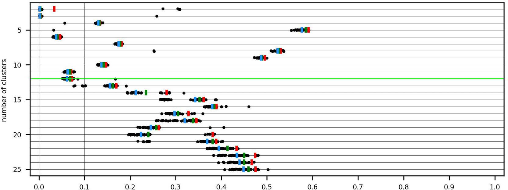
Figure 10 displays the distributions of normalized CMER for the 12-clustering. The two smallest clusters, 8 and 11, are unstable. Their data lines are highlighted red because CMER = 1 with all samples. The remaining clusters are stable. The clustering is admissible for downstream analysis because the unstable clusters have fewer than 500 cells. The blue, green, and red lines extending from the bottom to the top of the plot indicate the median, 75th, and 90th percentiles of MED for the clustering.

Cell assignments to the ten k-means clusters summarized in Figure 3 of the paper [18] are evidently not publicly available. To attempt to compare clusterings found by our method with published results, the input data (68,579 cells) were clustered (k-means) using code from a 10x Genomics Github repository (see the section “Data and software availability” below). The sizes of the 10 clusters we obtained do not agree with the percentages in Figure 3b (nor is it obvious how these clusters correspond to the ones discussed in the paper). In particular, we obtained one small cluster – of 176 cells. The remaining 9 clusters range in size from three thousand to eighteen thousand cells. When the clusters obtained with our process were matched to these, none of the 176 cells in the smallest cluster were included – filtering discarded all of them.
Table 12 compares the 9 k-means clusters with the 12 hierarchical clusters. The adjusted Rand index equals 0.55.
- The majority of cells in k-means cluster 10 are split three ways. Most are in hierarchical cluster 7, which is stable. Approximately 300 cells each are in clusters 8 and 11, which are unstable.
- K-means cluster 9 is split four ways. Cells are divided among hierarchical clusters 0,1,9, and 10. Differential expression may help determine if these clusters are meaningful or spurious.
- K-means clusters 6 and 1 correspond to hierarchical clusters 2 and 3, respectively.
- 60% of the cells of k-means cluster 5 account for 80% of hierarchical cluster 6.
- 95% of cells in k-means cluster 4 are grouped with 90% of the cells in k-means cluster 7 in hierarchical cluster 5.
- 90% of cells in k-means cluster 2 are combined with nearly all of k-means cluster 3 and cells from other clusters into hierarchical cluster 4.
We review a second analysis of the 68k PBMC data because it yields a clustering more compatible with the k-means clusters. It is the result of the third iteration described in section 2.8. After deleting outliers, 63,281 cells were retained. Figure 11 displays the distributions of normalized MED. Only the 2 and 3-clusterings are stable.
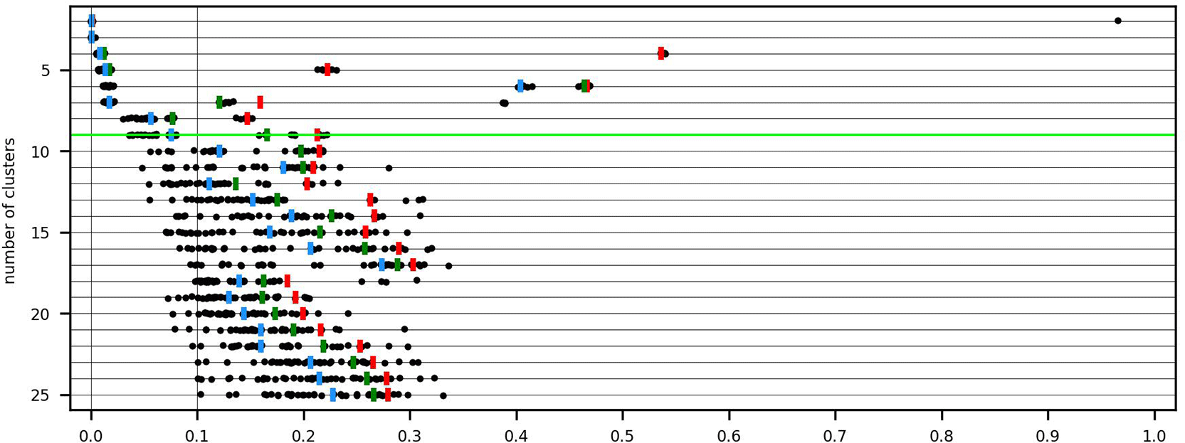
Preliminary exploratory analysis using the median of MED instead of the 90th percentile to define stable clusterings led to consideration of the 9-clustering (green highlighted line) because it is the largest with median MED (blue marker) less than or equal to 0.10. It fails to satisfy the criterion we now propose to define a stable clustering. The 90th percentile of MED equals 0.21.
The confusion matrices in Tables 2 and 3 are for two of the samples summarized in Figure 12, which displays the distributions of normalized CMER for the 9 clusters.

Cluster 3 (top line) is unstable. CMER = 1 with 39 samples. Cluster 1 (6th line) is also unstable. The 75th percentile of normalized CMER equals 1. Cluster 6 is unstable by a narrow margin. The remaining clusters are stable.
Table 13 compares the 9 k-means clusters with the 9 hierarchical clusters. The adjusted Rand index equals 0.66.
- Most of the cells in the unstable cluster 3 belong to k-means cluster 1. Recall that almost all of the cells in the two unstable clusters of the 12-clustering belong to k-means cluster 10.
- Each k-means cluster except 3 is unambiguously associated with a hierarchical cluster.
25k retinal
The counts downloaded from the Gene Expression Omnibus contain data for 49,300 cells. We followed Lause et al. [19] by restricting to replicates p1 and r4-r6, netting counts for 22,292 genes and 24,769 cells. Thirty-nine cell clusters were reported ( Figure 5D of) [20]. Restricted to the cells we analyzed, cluster sizes range from 14 to 15,709 cells.
Filtering to exclude genes with nonzero counts on fewer than 50 cells retained 13,552 genes. Because data were not input through Seurat, cells were not screened for high mitochondrial DNA levels. 1,081 genes were found to be highly variable in the full data set and in all 40 samples.
The rank of the Pearson residuals matrix was estimated as 51 by optht. After mapping to a 51-dimensional SVD representation and excluding kNN outliers, 24,101 cells were retained. These cells belong to 37 of the 39 reported clusters.
Our objective was to evaluate clusterings of sizes 2–70 – the largest being greater than the number of reported cell clusters (39). The stopping conditions limited the largest clustering for at least one sample to a smaller size: 61 for iteration 1, 62 for iteration 2, 58 for iteration 3.
The largest stable clusterings found in the first and second iterations have 5 clusters. The largest stable clustering found in the third iteration has 11. The third iteration retained 22,416 cells, which belong to 36 of the 39 published cell clusters.
Figure 13 displays the distributions of normalized MED for the clusterings of sizes 2–58 found with the third iteration.
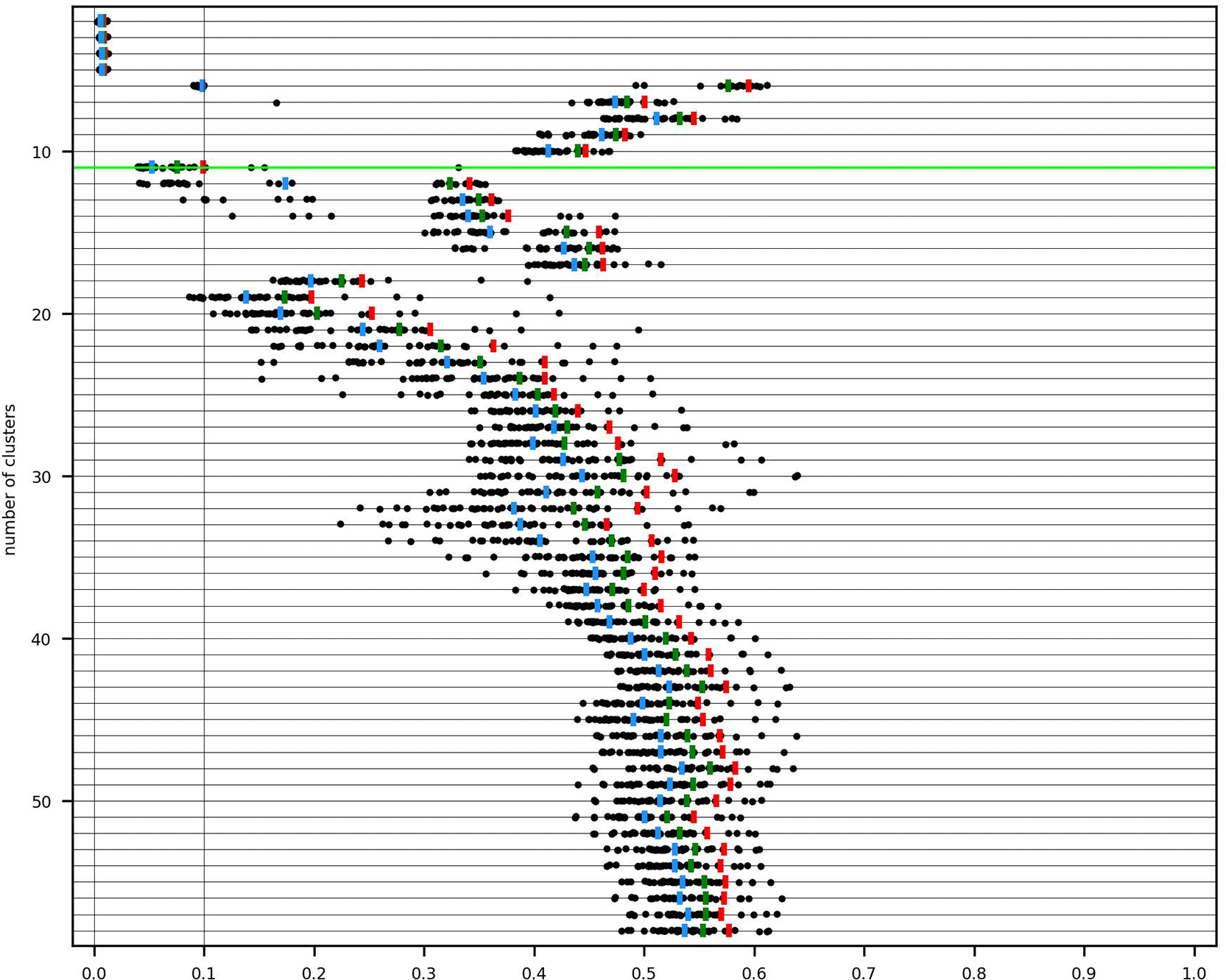
Figure 14 displays the distributions of normalized CMER for the 11 clusters. Cluster 9 is unstable. Because CMER = 1 with all samples, the line is marked red. Cluster 6 is also unstable. The remaining clusters are stable. The clustering is admissible for downstream analysis.

Table 14 illustrates the compatibility of the 11 hierarchical clusters with the reported cell clusters. The adjusted Rand index equals 0.49.
- Most members of cell cluster 24 (rods) belong to hierarchical clusters 0 and 1. We anticipate using differential expression analysis to evaluate this split.
- Similarly, cell cluster 26 is split between hierarchical clusters 2 and 3.
- Cell cluster 25 (cones) agrees closely with hierarchical cluster 8.
- Cell cluster 3 agrees almost exactly with the unstable hierarchical cluster 9.
- 80% of the cells in cluster 27 belong to the unstable hierarchical cluster 6.
- Cell cluster 34 agrees closely with the very stable hierarchical cluster 10.
65k lung
The paper [22] describes separately clustering the data for each patient. Our analysis included batch correction. Each patient’s data were treated as an independent batch.
The data set contains counts for 26,485 genes and 65,662 cells. The accompanying metadata file provides 57 cell type annotations.
Excluding data for blood cells retained 60,993 cells. Filtering to exclude genes with nonzero counts on fewer than 50 cells retained 17,470 genes. Because data were not input through Seurat, cells were not screened for high mitochondrial DNA levels. 1,659 genes were found to be highly variable in the full set of data and all 40 samples.
The rank of the Pearson residuals matrix was estimated as 305 by optht. After mapping to a 305-dimensional SVD representation and excluding kNN outliers, 60,114 cells were retained.
Our objective was to evaluate clusterings of sizes 2–70 – the largest being greater than the number of reported cell types (57). The stopping conditions limited the largest clustering for at least one sample to a smaller size: 69 for iteration 1, 48 for iteration 2, 41 for iteration 3. The largest stable clustering found in the first iteration has 19 clusters. The largest stable clusterings found in the second and third iterations have 13 clusters.
Figure 15 displays the distributions of normalized MED for the clusterings of sizes 2–69 found with the first iteration. The green lines highlight data for the clusterings of sizes 16 and 19, which are reviewed.
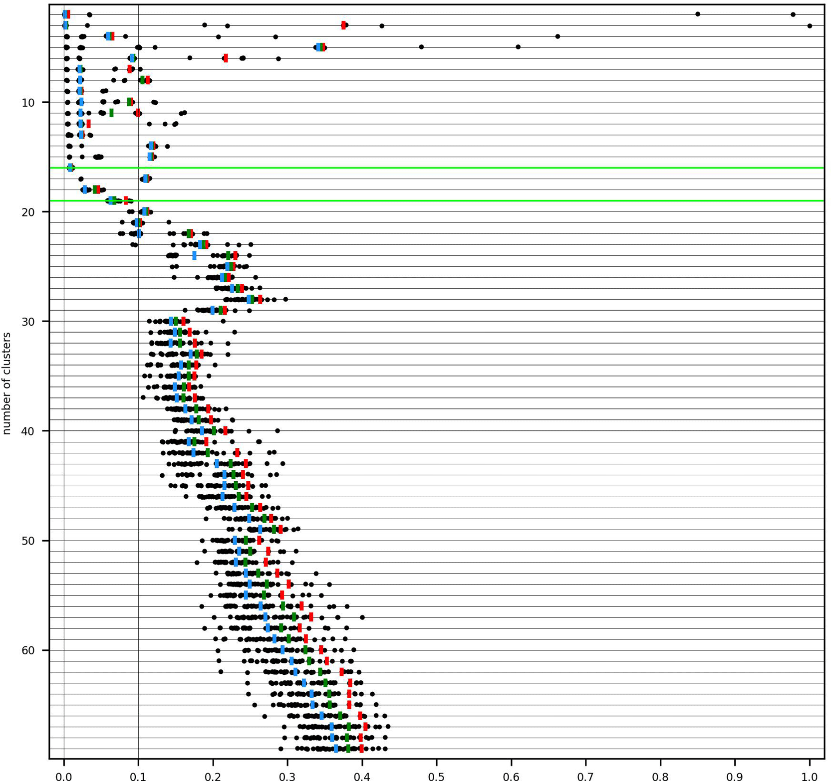
Figure 16 displays the distributions of normalized CMER for the 19 clusters. Clusters 1 and 4 (first and third lines) are unstable. The remaining clusters are stable. The clustering is admissible for downstream analysis.
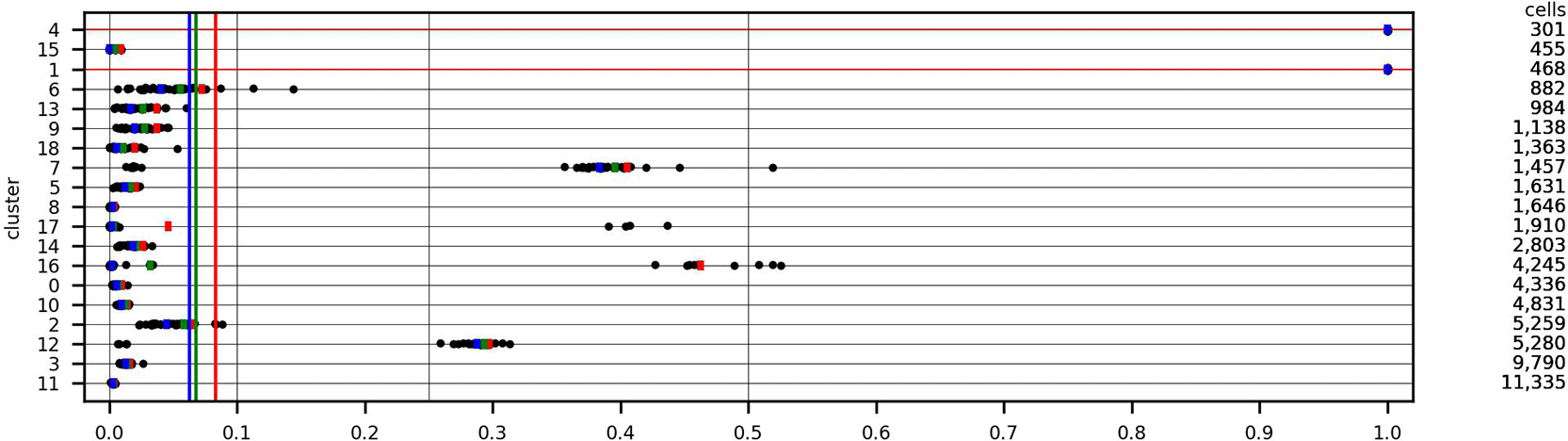
Because blood cells were excluded from our analysis, data for one cell type were eliminated. Table 15 illustrates the compatibility of the 19 hierarchical clusters with the 56 retained cell types. The adjusted Rand index equals 0.65. The majority of macrophages are divided between clusters 2 and 3.
The 16-clustering of the same data is reviewed because the results – for both the clustering and its clusters – are the most stable found in the four large data sets. Referring to Figure 15, the maximum value of normalized MED equals 0.01. We cannot explain this why it is exceptionally small.
Figure 17 displays the distributions of normalized CMER for the 16 clusters. All are stable.
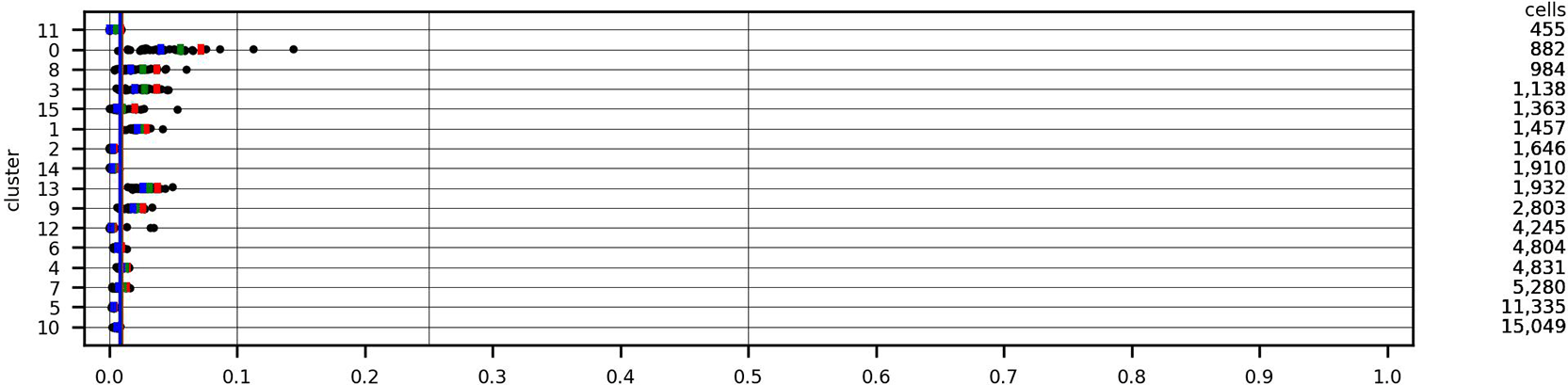
Table 16 compares the published cell types with the 16 hierarchical clusters. The adjusted Rand index equals 0.81. The majority of macrophages belong to cluster 10.
100k breast cancer
Discussion in [24] and programs posted at [40] suggest that batch correction was performed for each patient’s data for some, if not all, analyses. In our analysis, each patient’s data were treated as an independent batch.
The data set contains counts for 29,733 genes and 100,064 cells. Nine major cell types were reported, as well as 29 minor cell types and 49 cell type subsets.
Filtering to exclude genes with nonzero counts on fewer than 50 cells retained 21,354 genes. The data include cells for which up to 20% of counts are due to mitochondrial DNA. (The percentage exceeds 5% for half of the cells.) 1,704 genes were found to be highly variable in the set of counts for all cells and in all 40 samples.
The rank of the Pearson residuals matrix was estimated as 434 by optht. After mapping to a 434-dimensional SVD representation and excluding kNN outliers, 98,681 cells were retained.
Our objective was to evaluate clusterings of sizes 2–70 – the largest being greater than the number of reported cell type subsets (49). The stopping conditions limited the largest clustering for at least one sample to a smaller size: 58 for iteration 1, 39 for iteration 2, 51 for iteration 3. No stable clusterings were found. The smallest values found for the 90th percentile of MED are 0.15 (first iteration), 0.16 (second), and 0.107 (third).
Figure 18 displays the distributions of normalized MED for the clusterings of sizes 2–51 found with the third iteration. We review the 9-clustering, which has the smallest 90th percentile (0.107). This near miss from being judged stable illustrates a disadvantage of hard thresholds. We describe the clustering as marginally unstable.
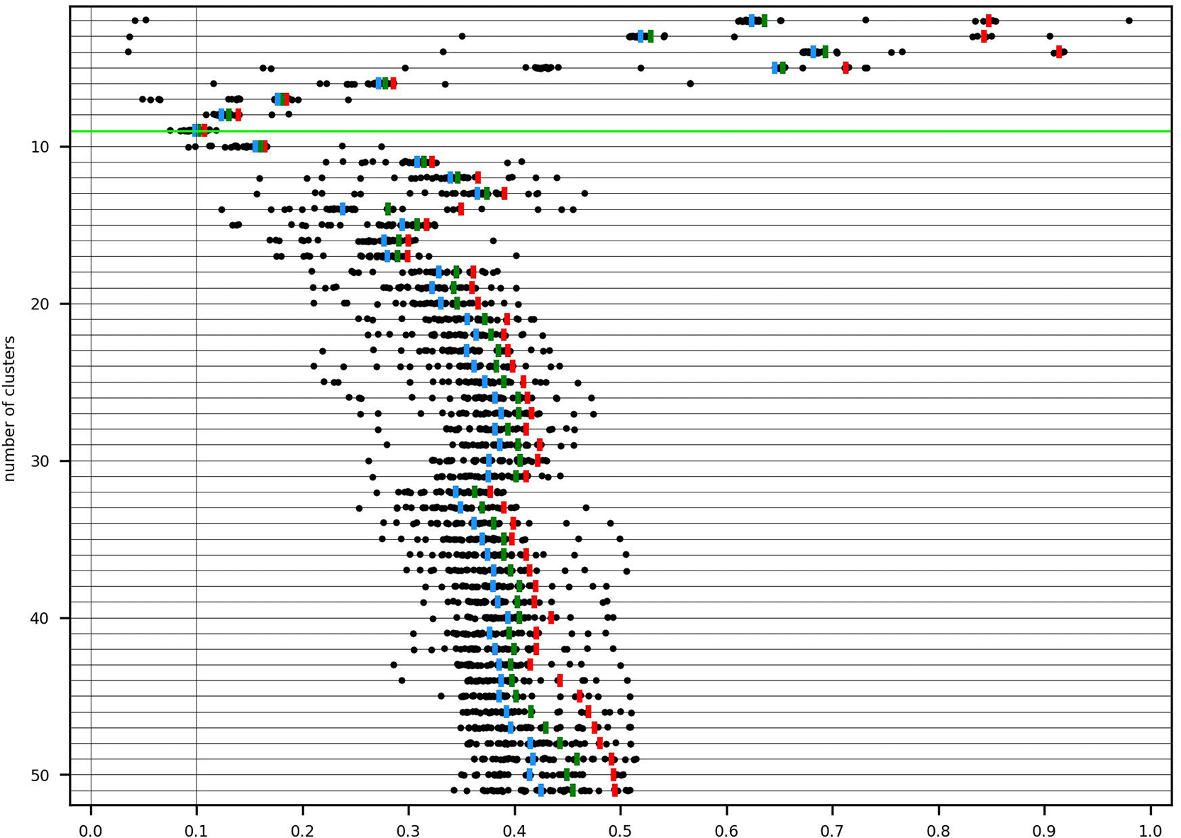
Figure 19 displays the distributions of normalized CMER for the 9 clusters. Cluster 6 (top line) is unstable. CMER equals 1 with 39 of the 40 samples. Cluster 0 (fifth line) is also unstable. The 90th percentile of CMER equals 0.55, larger than the threshold of 0.50 that defines stable clusters. This is a second reminder of the disadvantage of hard thresholding. The remaining clusters are stable. The clustering is not admissible for downstream analysis.

.
The third iteration retained 92,182 cells, which include all 49 published cell types. Filtering had a disproportionate impact on plasmablasts, one of the 9 major cell types. The data downloaded from the GEO included counts for 100,064 cells ( Table 1) of which 3,524 are plasmablasts. Excluding kNN outliers before clustering retained 98,681 cells ( Table 4) of which 2,290 are plasmablasts. They account for 1,234 of the 1,383 cells excluded as outliers in the first iteration. Only 801 plasmablasts were retained in the third iteration.
Table 17 compares the 9 hierarchical clusters with the major cell types. The adjusted Rand index equals 0.86.
- The hierarchical clusters do not separate normal from cancer epithelial cells, though approximately a quarter of the normal cells are assigned to cluster 2, accounting for more than 95% of its membership.
- The unstable cluster 6 represents a segment of myeloid cells.
- 90% of the plasmablasts that survived the filtering iterations are split between clusters 3 and 5.
Table 18 illustrates the compatibility of the 9 hierarchical clusters with the 49 cell type subsets identified in the paper. The adjusted Rand index equals 0.20.
- Cluster 2, mostly normal epithelial cells, corresponds to myoepithelial cells.
- Cluster 6 (unstable) corresponds to myeloid c4 DCs pDC IRF7 cells.