There has been an increasing literature regarding the adoption of GARCH models into an auditing model, particularly in the provisions of International Standard on Auditing (ISA) 570 with specific reference made to the banking and financial sectors. GARCH-based volatility modeling, pioneered by Engle et al. (2012) and Francq and Zakoian (2019) since, has been used to predict Value-at-Risk (VaR) and Expected Shortfall (ES), hence assessing audit risk.^1,2 Chaiyawat and Guayjarernpanishk (2024) have shown that multivariate GARCH models provide better insurer capital estimates, which underlines solvency analysis, which is a highly important task in the context of auditing.³ On the same note, Oskay et al. (2017) have highlighted the usefulness of GARCH models in ensuring that VaR predictions meet compliance with the regulation, which enhances the reliability of the audit.⁴

The importance of GARCH models in setting minimum capital requirements has been pointed out in other researches including those by Floros (2007) and Brooks et al. (2004), which is an indispensable component in the test of going-concern assumptions. However, the issue of volatility over estimation and model persistence has been raised and it highlights that there is a risk of errors in audit in case such models are not tested rigorously.^5,6 In their research, both Jin and Lehnert (2011) and Malone et al. (2009) used structural GARCH models to evaluate credit risk in situations of financial crisis and indicated that those models are best in predicting CDS spread although they have constraints when it comes to estimations in extreme situations.^7,8 Michański et al. (2023) and Contino and Gerlach (2017) at the methodological level studied hybrid GARCH-deep learning models and reported an enhanced predictive accuracy but still, there are difficulties in the implementation of hybrid GARCH-deep learning models into audit processes. Wallenstein (2023) also suggested the use of mixed-frequency GARCH modeling of high-frequency banking information to increase audit relevance.^9,10 Lin et al., and Elyasiani and Mansur (2004) revealed that multivariate GARCH models can identify risk contagion among bank portfolios and thus support the efforts by auditors to monitor systemic risk.^11,12

In addition, Zagonov et al. (2017) and Wymeersch (2012) emphasized the direct relevance of the GARCH models to ISA 570 and the ability of these models to increase the quality of the financial disclosure and to evaluate the resilience of firms. However, both articles found a gap of clear steps on how to incorporate GARCH results in the documentation of auditing, thus, making it a hindrance to the real implementation.^13,14 Greuning and Brajovic-Bratanovic (2004) have developed a correlation between governance-based risk-control frameworks and the results of audit.¹⁵

Overall, the reviewed twelve studies shed light on the consistent direction of introducing the advanced econometric models into the world of auditing, yet, the available literature lacks the standardized implementation procedures, particularly, the ability to align the interpretation gaps existing between the statistical results and the audit evidence requirements as outlined in ISA 570. This, therefore, highlights the need of further methodological improvement and training of auditors to realize the full potential of GARCH models in the audit environment.

The determinants of the capability of the company to remain in business are financial stability and market volatility. Professional judgment in auditing practice is a combination of quantitative models and professional judgment, which allows to improve the accuracy and reliability of professional judgment. Based on the importance of GARCH models in explaining the volatility, the study will present the following hypotheses to be tested empirically:

Companies are normally formed under the anticipation of indefinite survival. In this regard therefore, the preparation of the financial statements is supposed to be based on a number of underlying principles, the most important of which is the going-concern assumption. This supposition has impacts on accounting and auditing practice, and its legitimacy is supported by both accounting and operation data that show the products of the anxieties of a wide community of outside stakeholders.

2.1.1 Auditing and going concern

Given the economic conditions that an entity faces both in the financial and the non-financial dimension in which such a company operates, especially in an uncertain climate, the auditor is increasingly required- and in fact, in most occasions well armed- to evaluate and report on the capability or incapability of the entity to operate in the predictable future as a going concern. This requirement makes the auditor collect non-financial and financial substantive evidence, thus making it easier to make an informed judgment. It is worth noting that the auditor has no obligation to ensure that the entity is viable in future or foreseeing its liquidation. Instead, the auditor has a mandate to seek any warning indicators or triggers that may signal an adverse effect on the entity being a going concern, or which may forewarn liquidation, and to record such in the audit report that will be attached to the financial statements being prepared by the entity.¹⁶ The opinion of the auditor on the going-concern issues is important information to various users and beneficiaries and thus would inform their economic decision-making on the entity. The external auditor, acting in good faith on behalf of the shareholders, has the responsibility of determining whether the entity has the ability to continue its operations to the extent to which it can be predicted and present all the indicators of concern. This obligation is essentially connected with one of the principal standards of auditing conduct, or the principle of professional care. On the other hand, the auditor is not held accountable for these developments if signs of going concern risk only surface after the auditor has carried out routine processes and used the proper professional skepticism. The auditor’s opinion regarding the company’s financial accounts is nevertheless communicated in the audit report. If an appropriate conclusion has been made that another accounting basis is preferable, the auditor must explain whether these statements comply with generally accepted accounting principles (GAAP) and, if not, which basis was employed.¹⁶

A. The going concern assumption and its effects on the audit:

The going concern assumption is a fundamental accounting theory that states that a company will continue to exist for the foreseeable future, often at least twelve months after the financial statement date. This assumption is critical because it affects the value of assets and liabilities on the balance sheet, presuming that they would be recognized and settled in the usual course of operations. Nonetheless, it has had the greatest impact on the audit process, transforming a primitive accounting principle into a key focus of audit judgment and risk assessment.¹⁷ The auditor is responsible for determining whether management’s adoption of the going-concern assumption is justified. This entails the auditor following methodical actions and procedures to assist in establishing the conditions or occurrences that may call into question the entity’s capacity to continue as a going concern. According to Carson et al. (2013), this approach is fraught with difficulties, including management bias, economic uncertainty, and the inability to foresee future trends. When evaluating management’s risk-reduction strategy, the auditor should exercise a high level of professional scepticism and judgment. This kind of assessment has a decisive impact on final audit opinion, in the case of significant doubt that is not properly disclosed, the auditor must amend audit report, possibly putting a going-concern opinion (with such implications that have far-reaching effects on the relationship between the entity and investors, creditors and other stakeholders) (Carson et al., 2013).

ISA 570 establishes severe guidelines for an auditor’s responsibilities in the event that the audited organization is unable to continue operations. It specifies the measures that should be taken to implement the audit in such a case.

2.2.1 Objective of the standard

A key part of ISA 570, Going Concern, is to establish a structured approach to the auditor’s obligations in relation to management’s application of the going concern assumption in financial statement production. The standard must not only offer people with jobs, but also instruct them on how to fulfill those jobs. This includes the creation of methods for identifying circumstances, including symptoms, such as chronic operating losses, negative cash flows, and significant changes in management that may suggest considerable concern about the entity’s capacity to continue.¹⁸ Furthermore, ISA 570 specifies the auditor’s actions in situations where such issues occur, necessitating an objective evaluation of management’s repair measures. According to De-la-Hoz et al. (2022), an important part of the auditor’s professional skepticism is its influence on the due process, since the valuation will undoubtedly have an impact on the audit report. The standard guides the auditor in determining whether a material uncertainty exists and how to communicate that conclusion, such as with an unmodified opinion with a “Material Uncertainty Related to Going Concern” section or, alternatively, a modified opinion if disclosure is insufficient. This method helps make sure that what the auditor does really communicates a clear and honest picture to stakeholders about the financial status of the organization. It’s not just about checking the boxes anymore; it’s evolving into a more insightful analysis.

2.2.2 Indicators of going concern as per the standard

These indicators are typically separated into financial, non-financial and other factors.

Financial indicators

The Evaluation of Going Concern Based on Financial Indicators The financial indicators evaluated in analyzing the firm’s going concern are as follows:

Current liabilities exceeding current assets;

Long-term loans cannot be repaid or restructured, or the utilization of short-term borrowing to finance long-term projects is too expensive;

I. Negative changes in financial ratios II. Deferral or termination of dividend payments III. Failure to meet creditors’ obligations IV. Difficulty with loan covenants V. Inability to fund new product development or capital investments.

Furthermore, if suppliers and creditors want cash instead of credit, it may indicate liquidity issues and decreasing confidence from business partners, which is a symptom of difficulties for the company and suggests an inability to continue operations.¹⁹

3. Generalized autoregressive conditional heteroscedastic models GARCH(p,q)

In 1986, the statistician (Bollerslev) expanded the ARCH model to another model that provides for a more flexible displacement structure, known as the generalized autoregressive conditional heteroscedastic model (GARCH). The ARCH model’s conditional variance is a function of past square errors, but the GARCH model’s conditional variance includes both past squared errors and shifting conditional variances. The GARCH model is preferred over the ARCH model because it has fewer parameters.

The mathematical representation of the GARCH model is as follows:²⁰

where α0>0, βj≥0,j=1,2,…,q,αi≥0,i=1,2,….,p.

2-3-4 Nonlinear time series analysis methodology

The methodology for analyzing nonlinear models often follows the following steps:²¹

Each of the above steps will be studied in detail as follows:

2-3-4-1 Identification

In this stage the data analyzed from the models (ARCH, GARCH) represents the return series instead of the original series by using the following formula:²¹

From the above equation, the non-stationary of the mean in the original series is treated by making it completely stable in the mean, while relying on drawing the autocorrelation function to identify the model after ensuring the stationary of the series²²

2-3-4-2 Nonlinearity test

There are two ways to test for effects ARCH, GARCH:

1- Lagrange multiplier test

It is also called ARCH test, which was discovered by the scientist (Engle) in 1982, Where the presence or absence of heteroscedasticity is tested, depending on the test hypothesis that states:

H0=αi=0fori=1,2,…,pH1=αi≠0

If this hypothesis is achieved, it means that there is no effect of heterogeneity for variance. Considering that the series model ( at2 ) is as follows:

The calculated value is compared with the tabular value with a specific level of significance (α) and with a degree of (p). If the calculated value is less than the tabular value, we accept the null hypothesis, meaning there is no ARCH effect.²³

2-Portmanteau Q statistics test

In 1978, the two scientists (Ljung-Box) modified the (Box and Pierce) test, which was proposed in 1970. this test is based on calculating the autocorrelation coefficients for the residuals under the hypothesis that:

H0:ρ1=ρ2=ρ1…=ρk=ρm=0∀k=1,2,…..,mH1:ρ1≠ρ2≠…≠ρk≠ρm≠0

The test is:

Where n is the sample size, m is the largest displacement of ln (n), and p is several model parameters

ρ̂k2 Estimates of autocorrelation coefficients for the series of residuals.

The value of Qm is compared with the value of xm−p2 and at a certain level of significance (∝). If the value of the test statistic is less than the value of xm−p2 We accept the null hypothesis, meaning there is no effect of heterogeneity. That is, there is no ARCH effect.²⁴

Estimation

There are several methods for estimating the parameters of nonlinear models, the most important of which is the maximum likelihood method, which is used in estimating the conditional variability models that proceed from the assumption that the errors have a certain distribution and is often a normal distribution. The two scientists (Bollerslev & Wooldridge) showed in 1992 that the estimates of the maximum likelihood of the GARCH models assume that the errors are normal, consistent even if the real distribution of the residuals is not normal.²⁵ Therefore, the researchers presented the estimation under the assumption of a normal distribution of errors to obtain consistent estimators.²⁶ The maximum likelihood function for ARCH (p) model provided that the errors are normally distributed:

f(x1,x2,⋯,xn|α_)=f(xn|Fn−1)f(xn−1|Fn−2)…f(xp+1|Fp)f(x1,⋯,xp|α_)(x1,x2,⋯,xn|α_)=∏t=p+1n12πσt2exp[−xt22σt2]∗f(x1,⋯,xp|α_)

where α_=[α0,α1,…,αp] , f(x1,⋯,xp|α_) Common probability density function for values x1,⋯,xp

Taking the logarithm, the function becomes in the following form:

L(α_)=∑t=p+1n[−12ln(2π)−12ln(σt2)−xt22σt2]

Since the first term does not include any parameter (i.e a fixed term), the logarithm of the maximum likelihood function is:

L(α_)=∑t=p+1n[−12ln(σt2)−xt22σt2]

Since the parameters in the vector (α_) are estimated by maximizing logarithm of the likelihood function. Estimating model parameters GARCH (p, q) is done by using the maximum likelihood function, as is the case in the ARCH model, assuming that the errors follow a normal distribution, where the parameter vector is as follows:

α_=[α0,α1,…,αp,β1,β2,…,βq]

Test the order of model

Choosing the model’s order is critical, as selecting a lower order than the real order results in inconsistencies. Choosing a higher order than the real and actual order increases the variance of the model, resulting in a loss of accuracy due to the increased number of parameters for the chosen model. Several criteria have been established to determine the order of ARCH and GARCH models, including (BIC, AIC).²⁷

Verification of the model

After estimating the parameters of the (ARCH, GARCH) models, the model is checked to show its suitability to the data of the studied series to carry out the most important process, which is the forecasting process, as we examine the series of standard residuals according to the following formula:

whereas x~tis a series of Standard Residuals, x̂t the series of residuals is estimated according to the equation x̂t=yt−û , σ̂t the series of conditional standard deviations is calculated from the square root of a model formula equation (GARCH) after the parameter estimation process.²⁸

To check suitability, use the Ljung-Box test on the standard series of residuals to indicate the mean equation, the square of the residual series to indicate the residual equation, or the ARCH test on the x~t series to indicate the instability equation (volatility).²⁹

Forecasting

It is the final step of the time series analysis, which cannot be achieved without passing the model through all diagnostic tests and tests to confirm the validity of the model used in the forecasting, and the following is an explanation of the forecasting process for models (ARCH, GARCH):

So:

1-step-ahead forecast of σh+12 h represents the original, and h = t-1

σh+12=σh2(1)=α0+α1ah2

2-step-ahead forecast is

σh2(2)=α0+α1σh2

The ℓ-step-ahead forecast of σh+ℓ2

σh2(ℓ)=α0+α1σh2(ℓ−1)

If ℓ−1≤0 then:

σh2(ℓ−1)=ah+ℓ−12

whereas: ℓ>1

The empirical data for this study is based on the closing share prices of Al-Taif Islamic Bank, which are listed on the Iraq Stock Exchange on a daily basis. The sample period runs from January 2, 2025 to June 30, 2025, during which time the region has political and economic instability, which influences market volatility.

Daily log returns are used to prepare data for volatility modeling yt were calculated using the natural logarithm of consecutive closing prices, according to the following equation:

yt=lnPt−lnPt−1

Where:

Pt : is the closing price of Al-Taif Islamic Bank on day t

Pt−1 : is the closing price on the previous trading day t−1

Days without trading were excluded from the series, resulting in a total of 180 valid observations.

The descriptive data of the daily log returns of the stock of Al-Taif Islamic Bank are shown in Table 1. With a mean return of 0.6083, the sample period appears to have had positive average performance. The comparatively high standard deviation (0.7706) suggests significant return volatility, which bolsters the case for using the GARCH and ARCH models.

Additionally, a broad range of daily return swings are reflected by the smallest value of 0.02 and the largest value of 4.56, which could be indicative of notable trading pressures or market reactions throughout the studied time.

The volatility dynamics during the study period were analyzed. A graphical representation of the Al-Taif Islamic Bank stock’s daily log returns, denoted as y, from January 1, 2025, to June 30, 2025, is illustrated in Figure 1, So there are noticeable spikes in both positive and negative directions as the returns swing around a zeroes mean. These spikes represent days with abnormally large price fluctuations caused by trading news, market shocks, or changes in liquidity. These types of oscillations are common in financial time series and lend credence to the concept of volatility clustering, which states that high volatility is followed by even higher volatility, and low volatility does the same.

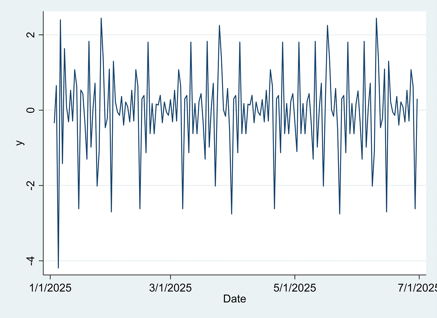
Significantly, the chart displays extreme values numerous times, including abrupt negative returns close to −4 and positive returns more than 2. These could be related to systemic or market events that have an impact on the banking industry or the broader Iraqi financial market during the research period.

All things considered, the trend in Figure 1 supports the use of ARCH/GARCH models, which are intended to represent the fluctuating variance (heteroskedasticity) in financial return series across time.

The Augmented Dickey-Fuller (ADF) unit root test was used to assess the stationarity of Al-Taif Islamic Bank’s return series y_t. This test is often used in time series analysis to see if a series has a unit root, which indicates non-stationarity.

The test was performed with Stata, and the results are shown in Table (2) below:

The return series y was checked for stationarity with the Augmented Dickey-Fuller (ADF) test, as shown in Table 2. The test’s null hypothesis states that the series is non-stationary because it has a unit root; the test statistic of −14.242 at the 1% (−3.484), 5% (−2.885), and 10% (−2.575) significance levels is significantly less than the critical values, and the MacKinnon estimated p-value of 0.0000 provides strong statistical support for the null hypothesis. This finding demonstrates that the return series is stationary, which means that its variance and mean do not fluctuate over time. This is significant because it supports the applicability of time series models such as GARCH and ARCH, which require stationarity as a basic criterion.

Upon confirmation of stationarity, the Lagrange Multiplier (ARCH-LM) test was performed with EViews 12 to detect the presence of ARCH effects in residuals. The null hypothesis states there is no ARCH impact (i.e., homoskedasticity).

Table 3 shows that the F-statistic is 17.3498 with a p-value of 0.0000, and the Obs*R-squared statistic is 14.7569 with the same p-value of 0.0000. These data are highly significant at the 1% level, hence the null hypothesis is rejected. This reveals significant evidence of conditional heteroskedasticity in the return series, which supports the use of ARCH and GARCH models to accurately capture time-varying volatility.

The results in Table 4 give compelling evidence against the null hypothesis of no serial connection in the return series yt . The p-values for all investigated lags (10, 15, 20, 25) are less than 0.05, showing that the residuals show statistically significant autocorrelation at each level. This shows that the return series is not completely random and has serial dependence.

Such strong autocorrelations show that the volatility of daily closing prices for Al-Taif Islamic Bank across the study period is time-dependent, with volatility clustering most certainly occurring. This means that high volatility is typically followed by high volatility, and vice versa, a key feature of financial time series.

The findings support the adoption of sophisticated volatility models like ARCH and GARCH, which are specifically designed to capture conditional heteroskedasticity and non-linear relationships in financial returns.

At this point, the parameters of conditional heteroskedastic autoregressive models were estimated while assuming non-constant error variance. These include the ARCH and GARCH models, which were tested to establish the optimum model for representing the data. The greatest likelihood method was employed to estimate the data, and numerous model assumptions were examined. The models were evaluated on the assumption that the residuals are normally distributed. Tables 5 and 6 present the results.

The Table 5 illustrates the estimation results of ARCH models for orders 1–4, which are aimed to represent volatility clustering in the return series. Across all models, the constant variance term (α₀) is extremely significant (p = 0.000), indicating strong unconditional variance in the series. The ARCH terms (α₁ to α₄), which measure the impact of prior squared residuals on current volatility, are consistently minor across all specifications. For the ARCH(1) model, the α₁ coefficient is estimated as 0.0756 with a p-value of 0.548, showing no significant ARCH effect. Similarly, higher-order terms in ARCH(2) to ARCH(4) are statistically insignificant, with p-values considerably above 0.05.

Using the Akaike Information Criterion (AIC) and the Bayesian Information Criterion (BIC), the ARCH(1) model is identified as the best option among the alternatives. It has the lowest AIC (551.0682) and BIC (560.6304), indicating that the model fit and complexity are optimally balanced. Although all models have the same log-likelihood values, the marginal advantages in fit from adding more lags do not exceed the additional parameters in terms of information requirements.

Overall, despite the statistical insignificance of the lagged ARCH terms, the ARCH(1) model is the preferable specification since it is simpler and performs better. The poor explanatory power of previous shocks may imply that volatility dynamics in this return series are better represented by more advanced models, such as GARCH variants, which integrate both ARCH and GARCH components to account for persistent volatility behavior more effectively.

Table 6 displays four distinct GARCH models, together with their estimated coefficients and model selection statistics: GARCH(1), GARCH(2), GARCH(2,1), and GARCH(2). The GARCH(2,2) outperforms the others in both the Akaike Information Criterion (AIC = 504.6756) and the Bayesian Information Criterion (BIC = 523.7999), with the best trade-off being between model fit and complexity.

The coefficients show a large constant variance term (α₀) for all models with p-values equal to 0.000, indicating a significant level of volatility in the series. ARCH effects (α₁ and α₂), which explain short-run volatility clustering, are substantial in the more complicated models, i.e., GARCH(2,1) and GARCH(2,2). Both α₁ and α₂ are significant at the 1% level.

In contrast, the GARCH(1,1) model produces unimpressive ARCH and GARCH coefficients (p > 0.05), indicating little explanatory power. Similarly, GARCH(1,2) outperforms GARCH(1,1) but trails GARCH(2,1) and GARCH(2,2). The GARCH parameters (β₁ and β₂), indicators of time-persistence in volatility, are statistically significant across all the models where they exist, especially for GARCH(2,2). This indicates that the volatility process of the data has high memory.

At this point, the best-fitting model will be selected and used to forecast future volatility. The model with the lowest AIC, BIC, and Log-Likelihood values, as well as the statistical significance of the calculated parameters, will be chosen. In addition, the greatest log-likelihood value will help in model selection. Table (7) displays the competing models, estimated parameters, log-likelihood values, and information criteria values (AIC, BIC, Log-Likelihood) based on the distribution of the model’s residual errors.

Table 7 clearly indicates compares the best ARCH and GARCH models, revealing considerable variations in their ability to capture the volatility structure of the return series. The ARCH(1) model has little explanatory power, as the ARCH coefficient (α₁ = 0.0756) is statistically insignificant (p = 0.548), and all other lags are removed. The GARCH(2,2) model has substantial statistical significance for all parameters, including ARCH terms (α₁ = 0.1486, α₂ = 0.1503) and GARCH terms (β₁ = −1.9590, β₂ = −1.0306), with p-values of 0.000. This suggests that both short-term shocks and long-term volatility persistence contribute significantly to the series’ variance.

Furthermore, the model selection criteria highly support the GARCH(2,2) model. The model has a higher log-likelihood value (−246.34 vs. −272.53) and lower AIC (504.68 vs. 551.07) and BIC (523.80 vs. 560.63) than the ARCH(1) model. These measurements indicate that GARCH(2,2) not only fits the data better, but also more efficiently, balancing complexity and performanceTo wrap up, while the ARCH(1) model offers a simplistic view of volatility, it can be depicted as a much better fit and statistical model of the conditional variance process of the return series when using the GARCH(2,2) framework.

Of all the models, it exhibited the best fit for the data and is therefore used to forecast future volatility of the series.

To forecast volatility of the daily closing prices of AI-Taif Islamic Bank over the study period, the GARCH(2,2) model was selected as the most suitable specification for the reasons of upfront explanations of the statistical significance of the estimated parameters and information criteria (AIC = 504.6756, BIC = 523.7999), which were the best levels of all competing models. The general form of the model is presented in:

yt=μ+rtrt=σtεtσt2=α0+α1rt−12+α2rt−22+β1σt−12+β2σt−22

By substituting the estimated parameters, the fitted model becomes:

yt=−0.0497+rtrt=σtεtσt2=5.1417+0.1486rt−12+0.1503rt−22−1.9590σt−12−1.0306σt−22

All estimated coefficients were statistically significant at the 1% level ( p -values =0.000 ), indicating a strong effect of past shocks and volatility on current conditic.al variance. Compared to ARCH models, the GARCH(2,2) specification offers a more robust and dynamic structure for modelling volatility persistence in the return series.

After identifying the optimal model and determining its order, and estimating the conditional variance series for the daily closing index of the Iraq Stock Exchange, it is essential to confirm the model’s adequacy and efficiency. This is done by applying the Ljung-Box and ARCH-LM tests on the standardized residuals and their squares, as mentioned during the model identification stage. The Ljung-Box test is applied to the residuals to test for autocorrelation, while the ARCH-LM test is used to examine the presence of any remaining ARCH effects. The statistical significance of these tests helps determine the adequacy of the model. Tables (8) and (9) present the results of these tests applied to the residuals and squared residuals of the GARCH(2,2) model.

Table 8 shows the results of the Portmanteau (Ljung-Box) test on the standardised residuals and squared values from the specified GARCH(2,2) model for lag lengths of 10, 15, 20, and 25. For all lag orders, the Q statistics are relatively low, with corresponding p-values of exactly 1.0000, significantly beyond the traditional significance threshold of 0.05. This demonstrates a significant failure to reject the null hypothesis of no serial correlation in both the residuals and their squared components. In other words, the residuals act as white noise, with no leftover autocorrelation or ARCH effects in the variance. These findings demonstrate that the GARCH(2,2) model well captures both the mean and volatility dynamics of the return series, demonstrating its applicability for modelling and predicting conditional variance.

Table 9 displays the ARCH LM test findings applied to the residuals of the fitted GARCH(2,2) model. The F-statistic is 0.15, with a p-value of 0.7019; the Obs*R-squared (Chi-squared test statistic) is 0.1485, with a p-value of 0.7181.

Both p-values are significantly higher than the typical 0.05 threshold, implying that we cannot reject the null hypothesis of no ARCH effects in the residuals. This means that there is no significant lingering ARCH-type heteroskedasticity in the residuals, indicating that the GARCH(2,2) model effectively captured the data’s conditional volatility structure. These findings corroborate the GARCH(2,2) model’s applicability and sufficiency in modeling the return series’ volatility dynamics.

Figure 2 approximate conditional variance of the GARCH(2,2) model and the conditional standard deviation of the stock returns of Al-Taif Islamic Bank between January–June 2025. The plot shows that there are obvious volatility clustering whereby there are high and low volatility periods that occur over time, hence supporting the existence of time-varying heteroskedasticity in the return sequence.

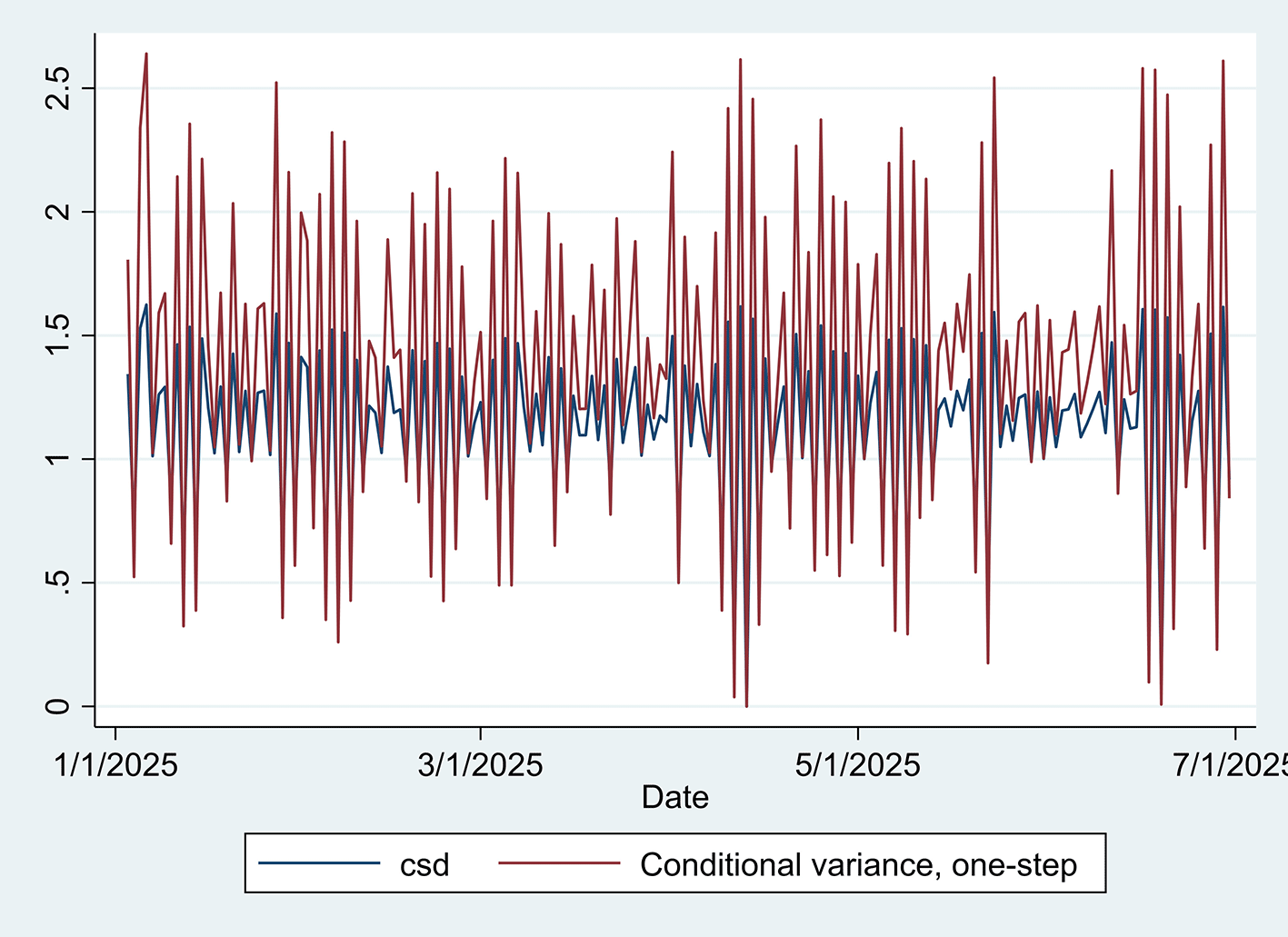
After identifying the appropriate model that best fits the time series data through the stages of diagnosis, estimation, and goodness-of-fit testing, the chosen model was used to forecast volatility. The In-Sample Forecasting method was used to forecast the daily closing price volatility, which was based on the estimated GARCH(2,2). In this method, volatility forecasting was conducted after selecting 275 observations (one-quarter of the sample), and the forecast was extended for 15 days. Table 10, as well as Figures 3 and 4, demonstrate this forecasting procedure.

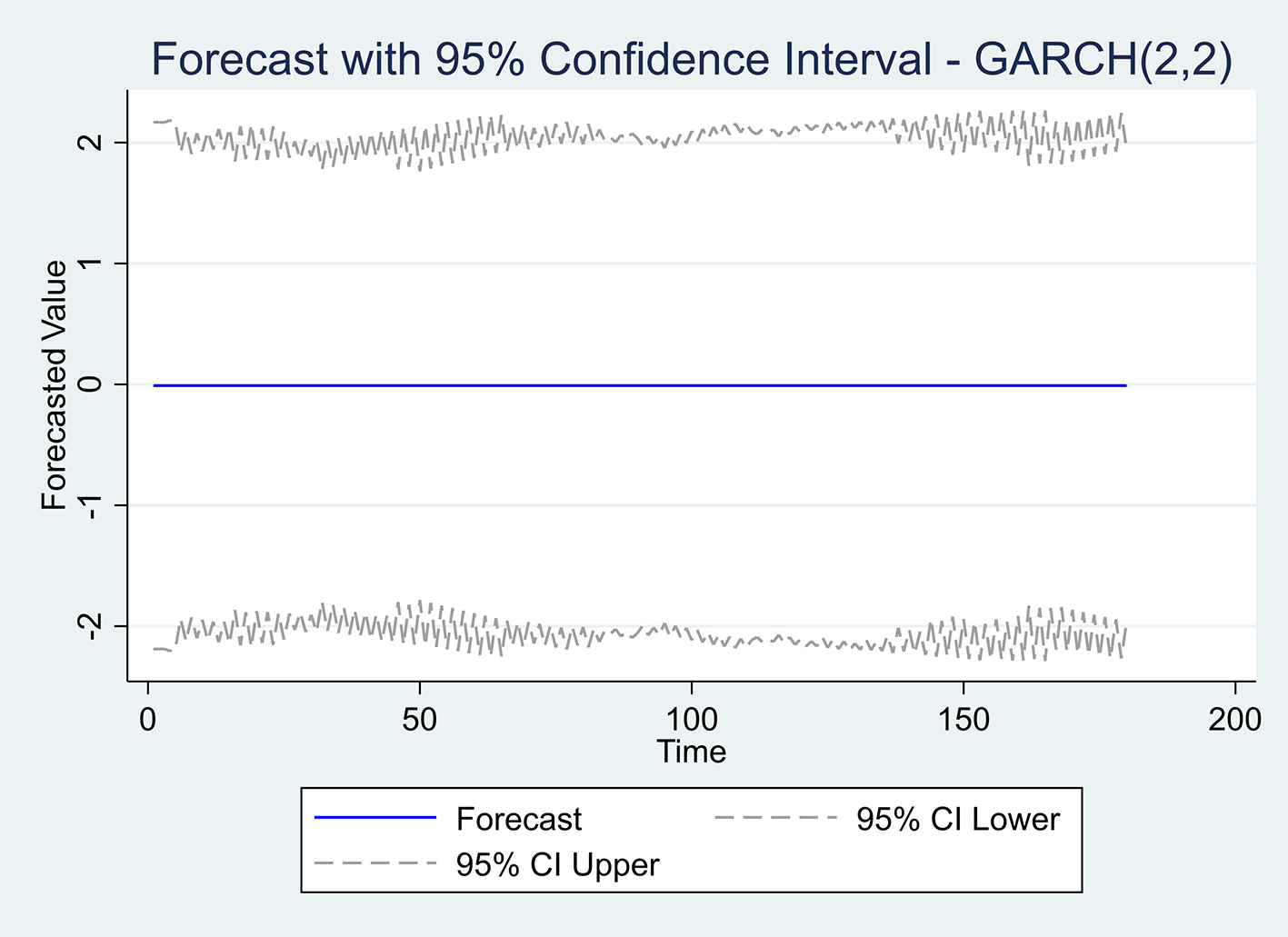
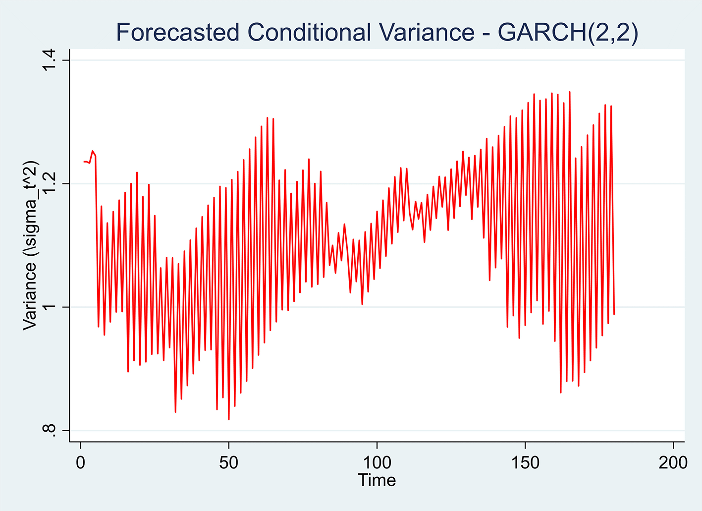
Table 11 summarizes the forecasting performance of the GARCH(2,2) model for Al-Taif Islamic Bank’s return series. The root mean square error is roughly 1.11, which reflects the average magnitude of forecast mistakes, with higher deviations receiving more weight. The mean absolute error is approximately 0.81, meaning that, on average, the forecast was less than one unit off from the actual readings. The mean absolute percentage error is roughly 10.75%, indicating that the model’s forecasts are wrong by about 10.75% on average when compared to the observed data. The low error values imply that the GARCH (2,2) model is reasonably fitted to volatility dynamics and forecasting ability for the entire period mentioned.

When examining Al-Taif Islamic Bank’s ability to continue as a going concern in accordance with ISA 570, the forecasting results from GARCH (2,2) provide useful information regarding the volatility behavior of the bank’s daily closing prices. The modest predicted results suggest good predictiveng abilities. The stated 95 percent confidence intervals and expected conditional standard deviations/variances provided an excellent match to the time-varying volatility data. According to ISA 570, auditors are required to determine whether there are any material uncertainties that could cast serious doubt on the entity’s capacity to operate as a going concern for the foreseeable future, which is typically defined as a period of twelve months from the date of the financial statements. An indirect indicator of market changes may be suggested by the expected volatility in this analysis that fluctuates only slightly and does not show sharp spikes or high sustained variance.

Nevertheless, it is important to merge statistical evidencetials with financial, operational, and macroeconomic analysis. Models of volatility by themselves are not an indicator of going concern status but do contribute to a fuller view of potential market variables that might influence the bank’s operations. Thus, given the predicted variance patterns at levels we can control, there is no clear signal of financial instability that would cause significant concern regarding going concern, based on ISA 570.

The implications of the results of this study have some serious policy and practical implications on the Iraqi auditing and regulatory environment. As the effectiveness of GARCH-based volatility modeling during the detection of financial instability has demonstrated, then it is possible to suggest that the quantitative methods can be a useful tool to the regulatory authorities as well as external auditors. In particular, the audit authorities of Iraq, such as the Federal Board of Supreme Audit and the Iraqi Association of Accountants and Auditors, may incorporate GARCH based volatility measures into risk based auditing models to enhance early warning mechanisms of financial distress. The realization of these econometric measures in planning audits allows auditors to assess the objectively determined market-driven risks that can threaten the survival of an entity as a going concern under the requirements of ISA 570.

Additionally, the volatility-driven models can be implemented by the supervisory bodies and other banking regulators, including the Central Bank of Iraq, to monitor the financial health of the banking organizations at any given time, and to record systemic risk factors before they turn into solvency issues. Such a data-driven method would not just increase the predictive success of risk assessment but it would also increase the transparency and credibility of audit reports. Eventually, the assimilation of GARCH-based tools in the regulatory and audit methods would bring the auditing standards in Iraq at par with the best global practices, thus developing higher confidence of the investors and the sustainability of the financial system in the long-term.