Просмотр новости
Найдите то, что Вас интересует
 Спутники
 РН
РН SpaceX
 Роскосмос
 NASA
NASA
СпутникиРНSpaceXРоскосмосNASAIn this tutorial, you’ll learn how vector databases achieve lightning-fast retrieval using Approximate Nearest Neighbor (ANN) algorithms. You’ll explore how FAISS structures your embeddings into efficient indexes (e.g., Flat, IVF, and HNSW), benchmark their performance, and see how recall and latency trade off as your dataset scales.

This lesson is the 2nd of a 3-part series on Retrieval-Augmented Generation (RAG):
To learn how to scale semantic search from milliseconds to millions of vectors, just keep reading.

In the previous lesson, you learned how to turn text into embeddings — compact, high-dimensional vectors that capture semantic meaning.
By computing cosine similarity between these vectors, you could find which sentences or paragraphs were most alike.
That worked beautifully for a small handcrafted corpus of 30-40 paragraphs.
But what if your dataset grows to millions of documents or billions of image embeddings?
Suddenly, your brute-force search breaks down — and that’s where Approximate Nearest Neighbor (ANN) methods come to the rescue.
In Lesson 1, we compared every query vector
against all stored embeddings  using cosine similarity:

If your dataset contains
vectors, this means  dot products for each query — an operation that scales linearly as
  .
.
That’s fine for 500 vectors, but catastrophic for 50 million.
Let’s do a quick back-of-the-envelope estimate:
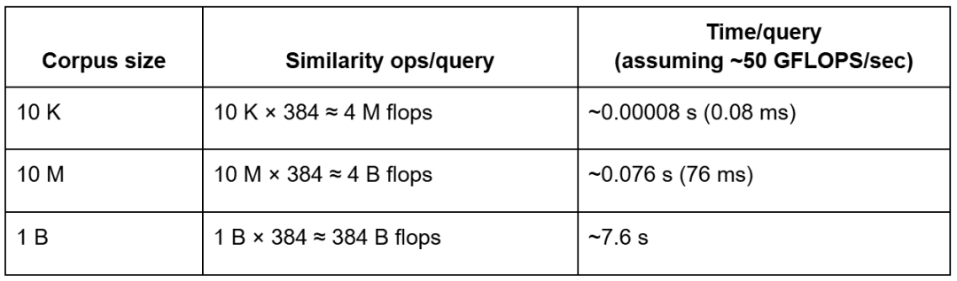 Table 1: Computational cost of brute-force cosine similarity as corpus size scales, assuming
 ᯈ50 GFLOPS/sec effective CPU throughput.Even on modern hardware capable of tens of gigaflops (GFLOPS) per second, brute-force search over billions of vectors still incurs multi-second latency per query — before accounting for memory bandwidth limits — making indexing essential for production-scale retrieval.
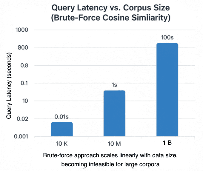 Figure 1: Brute-force cosine similarity scales linearly with corpus size, becoming infeasible beyond hundreds of millions of vectors (source: image by the author).
High-dimensional data introduces another subtle problem: distances begin to blur.
In 384-dimensional space, most points are almost equally distant from each other.
This phenomenon, called the curse of dimensionality, makes “nearest neighbor” less meaningful unless your metric is very carefully chosen and your embeddings are normalized.
🧠 Intuition: imagine scattering points on a 2D plane — you can easily tell which ones are close.
In 384D, everything is “far away,” so naive distance computations lose discriminative power.
That’s why normalization (L2) is critical — it keeps embeddings on a unit hypersphere, letting cosine similarity focus purely on angle, not length.
But even with normalization, you still can’t escape the sheer computational load of checking every vector.
So, how do we search faster without comparing against every vector?
Approximate Nearest Neighbor (ANN) algorithms do exactly that.
They trade a small amount of accuracy (recall) for huge latency gains — often 100× faster.
Conceptually, they build an index that helps jump directly to promising regions of vector space.
Think of it like finding a book in a massive library:
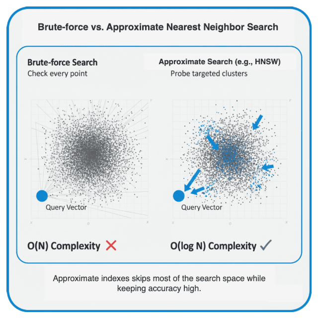 Figure 2: Approximate nearest neighbor methods (e.g., HNSW) skip most of the search space, dramatically reducing query time while maintaining high recall (source: image by the author).
ANN methods exist in many flavors — graph-based (HNSW), cluster-based (IVF), tree-based (LSH, KD-Tree), and hybrid approaches — but they all share a single philosophy:

They do so by:
You’ll often see performance expressed using recall@k, the fraction of true neighbors recovered among the top-k results.
A good ANN index achieves 0.9 – 0.99 recall@k while being orders of magnitude faster than brute force.
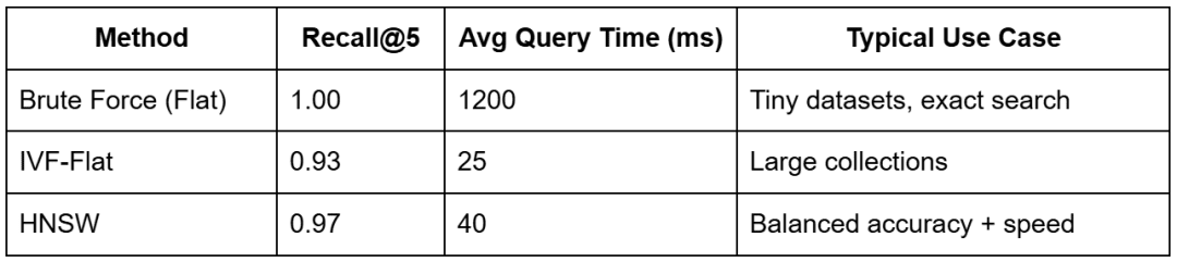 Table 2: Example recall and latency comparison of Flat, IVF-Flat, and HNSW indexes on a medium-scale corpus.
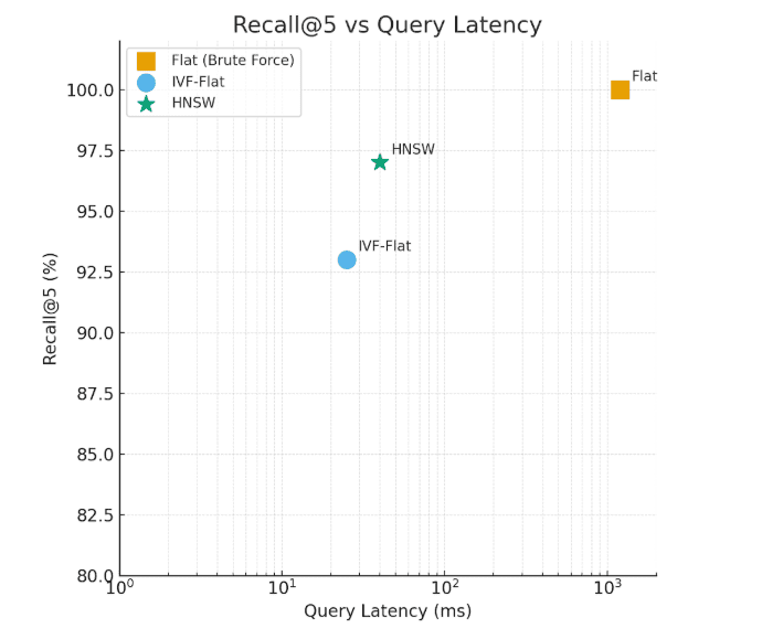 Figure 3: Approximate indexes (e.g., HNSW and IVF-Flat) achieve near-perfect recall while being orders of magnitude faster than brute-force Flat search (source: image by the author).
The Flat index delivers exact results but with high latency, whereas HNSW and IVF-Flat balance speed and accuracy for scalable retrieval.
In the next section, we’ll open the black box and look inside FAISS — the industry-standard library that powers vector search at scale.
You’ll understand how these indexes (i.e., Flat, IVF, and HNSW) are built, what parameters control their trade-offs, and how to construct them yourself in code.
By the end, you’ll see how these algorithms let you scale semantic search from a few dozen vectors to millions — without loss of meaning.
Would you like immediate access to 3,457 images curated and labeled with hand gestures to train, explore, and experiment with … for free? Head over to Roboflow and get a free account to grab these hand gesture images.
In Lesson 1, we learned how to generate embeddings and compute semantic similarity.
In Section 1 of this post, we discovered why brute-force search breaks down as our vector collection grows.
Now, let’s open the black box and explore how FAISS makes large-scale vector search practical.
FAISS (Facebook AI Similarity Search) is an open-source library developed by Meta AI for efficient similarity search and clustering of dense vectors.
It’s implemented in highly optimized C++ with Python bindings and optional GPU support.
In simple terms, FAISS is the NumPy of vector search — it provides a consistent interface for building, training, querying, and persisting vector indexes, with dozens of back-ends optimized for both accuracy and speed.
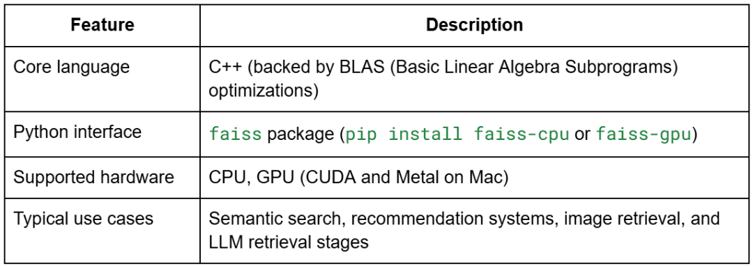 Table 3: Core components of FAISS for efficient approximate nearest neighbor (ANN) search.
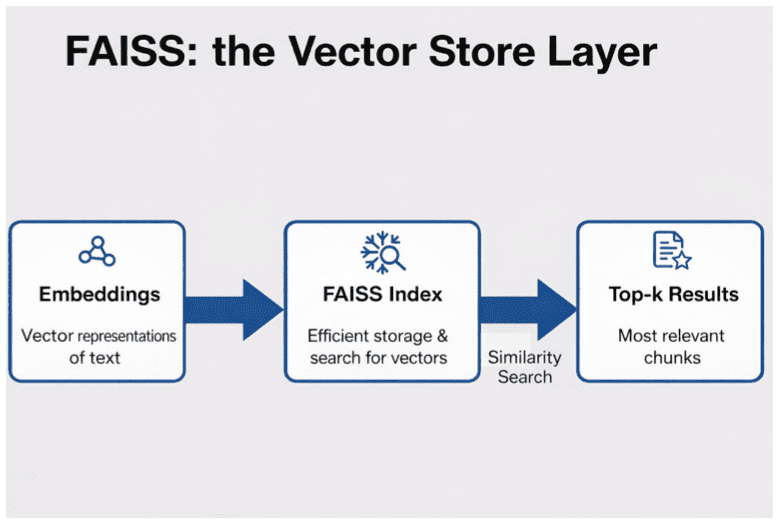 Figure 4: FAISS serves as a high-performance bridge between embeddings and retrieval logic, performing similarity search to return top-k relevant chunks efficiently (source: image by the author).
Every FAISS index is a data structure that helps you locate nearest neighbors efficiently in a large vector space.
Instead of storing raw vectors in a flat array and scanning them linearly, FAISS builds one of several possible structures that act as “shortcuts” through the space.
Let’s explore the three we will implement in this tutorial — Flat, IVF-Flat, and HNSW — and see how each balances speed and accuracy.
The Flat index is the simplest and most precise approach.
It stores every embedding as is and computes cosine similarity (or inner product) between the query and each vector.

This is essentially our brute-force baseline from Lesson 1.
It achieves perfect recall (1.0) but scales poorly — every query requires scanning all vectors.
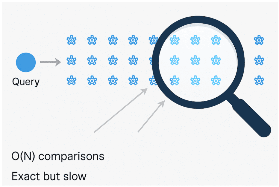 Figure 5: In brute-force vector search, each query is sequentially compared to every stored vector — an
 O(N) process that ensures exact matches but becomes prohibitively slow for large-scale datasets (source: image by the author).IVF stands for Inverted File Index.
The idea is simple but powerful: partition the vector space into coarse clusters and search only a few of them at query time.
Step-by-step:
nlist of them.nprobe of them (the most promising clusters).That reduces search complexity from O(N) to roughly O(N / nlist × nprobe).
 Table 4: Key configuration parameters of the FAISS IVF index and their impact on recall and search latency.
The Hierarchical Navigable Small World (HNSW) index uses a graph instead of clusters.
Each embedding is a node connected to its nearest neighbors.
At query time, the algorithm navigates the graph — starting from a random entry point and greedily moving to closer nodes until it reaches a local minimum.
This search is then refined by probing nearby connections to find better candidates.
 Table 5: Key HNSW parameters controlling graph connectivity and search-time accuracy-latency trade-offs.
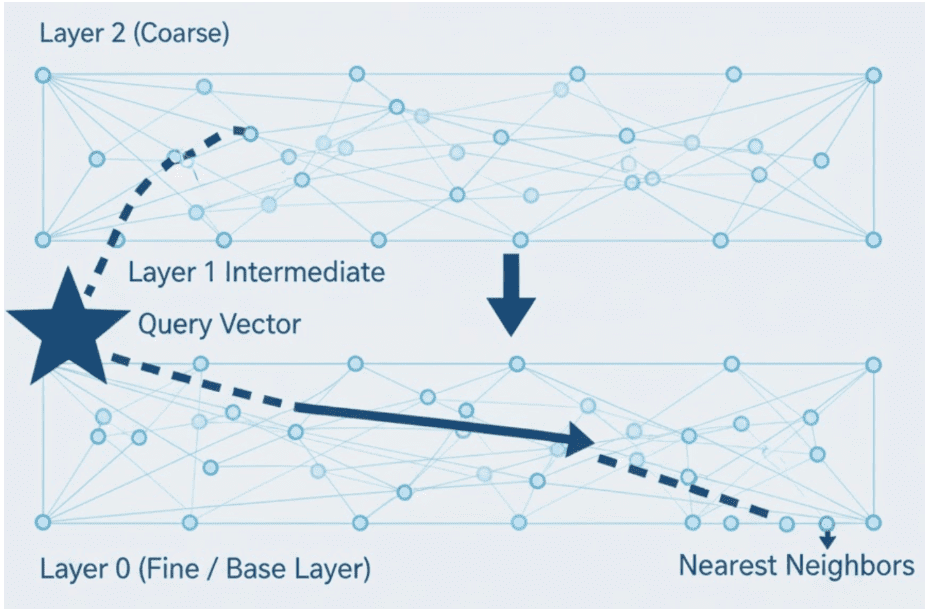 Figure 6: HNSW organizes vectors into multiple graph layers. The query starts at a coarse layer and navigates downward, refining its path at each level until it reaches the base layer to retrieve the nearest neighbors efficiently (source: image by the author).
Intuition: It’s like finding a friend’s house by asking neighbors for directions instead of checking every street yourself.
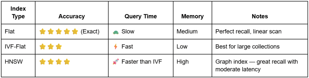 Table 6: Performance comparison of FAISS index types for approximate nearest neighbor (ANN) search.
Now that you understand what each index does, you’ll see how to implement them with FAISS.
In the next section, we’ll dive into the code — explaining config.py, vector_search_utils.py, then building and benchmarking indexes side by side.
To follow this guide, you’ll need to install several Python libraries for vector search and approximate nearest neighbor (ANN) indexing.
The core dependencies are:
$ pip install sentence-transformers==2.7.0
$ pip install faiss-cpu==1.8.0
$ pip install numpy==1.26.4
$ pip install rich==13.8.1
faiss-cpu for CPU-only environments (most common)faiss-gpu instead for better performance with large datasetsIf you plan to extend the examples with your own experiments:
$ pip install matplotlib # For creating performance visualizations
You can verify FAISS is properly installed by running:
import faiss
print(f"FAISS version: {faiss.__version__}")
 Having trouble configuring your development environment? Want access to pre-configured Jupyter Notebooks running on Google Colab? Be sure to join PyImageSearch University — you will be up and running with this tutorial in a matter of minutes.
All that said, are you:
Then join PyImageSearch University today!
Gain access to Jupyter Notebooks for this tutorial and other PyImageSearch guides pre-configured to run on Google Colab’s ecosystem right in your web browser! No installation required.
And best of all, these Jupyter Notebooks will run on Windows, macOS, and Linux!
Alright, time to get our hands dirty.
You’ve seen why indexing matters and how FAISS structures (e.g., Flat, HNSW, and IVF) work conceptually; now we’ll implement them and run them side-by-side. We’ll build each index, query it with the same vectors, and compare recall@k, average query latency, build time, and a rough memory footprint.
To keep things clean, we’ll proceed in 3 parts:
These constants keep paths, filenames, and defaults in one place, so the rest of the code stays clean and portable.
from pathlib import Path
import os

# Base paths
BASE_DIR = Path(__file__).resolve().parent.parent
DATA_DIR = BASE_DIR / "data"
INPUT_DIR = DATA_DIR / "input"
OUTPUT_DIR = DATA_DIR / "output"
INDEX_DIR = DATA_DIR / "indexes"
FIGURES_DIR = DATA_DIR / "figures"

# Corpus files (allow environment overrides for flexibility)
_CORPUS_OVERRIDE = os.getenv("CORPUS_PATH")
_CORPUS_META_OVERRIDE = os.getenv("CORPUS_META_PATH")
CORPUS_PATH = Path(_CORPUS_OVERRIDE) if _CORPUS_OVERRIDE else INPUT_DIR / "corpus.txt"
CORPUS_META_PATH = Path(_CORPUS_META_OVERRIDE) if _CORPUS_META_OVERRIDE else INPUT_DIR / "corpus_metadata.json"

# Embedding artifacts
EMBEDDINGS_PATH = OUTPUT_DIR / "embeddings.npy"
METADATA_ALIGNED_PATH = OUTPUT_DIR / "metadata_aligned.json"
DIM_REDUCED_PATH = OUTPUT_DIR / "pca_2d.npy"

# Index artifacts
FLAT_INDEX_PATH = INDEX_DIR / "faiss_flat.index"
HNSW_INDEX_PATH = INDEX_DIR / "faiss_hnsw.index"

# Models & defaults
EMBED_MODEL_NAME = "sentence-transformers/all-MiniLM-L6-v2"
SEED = 42
DEFAULT_TOP_K = 5
SIM_THRESHOLD = 0.35  # not used in this lesson, but fine to keep

# Ensure dirs exist
for d in (OUTPUT_DIR, INDEX_DIR, FIGURES_DIR):
    d.mkdir(parents=True, exist_ok=True)
What’s happening here (and why):
BASE_DIR and derive data/ subfolders so the repo runs the same on any machine.CORPUS_PATH and CORPUS_META_PATH can be overridden via environment variables — a nice quality-of-life touch if you swap datasets.EMBEDDINGS_PATH is the cache produced in Lesson 1; we load it here to avoid re-embedding.FLAT_INDEX_PATH and HNSW_INDEX_PATH are where we’ll persist FAISS indexes after benchmarking. (IVF can be added similarly if you want on-disk reuse.)Note: The file also contains prompt-related constants for Lesson 3 (RAG). We don’t use them here — safe to ignore in this lesson.
This module is your FAISS “Swiss Army Knife.” We’ll go through every function you shared, including the ones you asked me not to miss: brute_force_search, measure_latency, and estimate_index_memory_bytes, plus query/save/load.
try:
    import faiss  # type: ignore
except ImportError:
    faiss = None  # type: ignore

def require_faiss():
    if faiss is None:
        raise ImportError("faiss not installed. Please pip install faiss-cpu (or faiss-gpu).")
This is a friendly safety check. Any time we build or query an index, we call require_faiss(). If FAISS isn’t installed, you get a clear error with the exact package to install.
def build_flat_index(embeddings: np.ndarray):
    require_faiss()
    d = embeddings.shape[1]
    index = faiss.IndexFlatIP(d)
    index.add(embeddings.astype(np.float32))
    return index
What it does:
We create an IndexFlatIP, where IP = inner product. Because our embeddings are L2-normalized (from Lesson 1), inner product equals cosine similarity. We then .add() all vectors (as float32) to the index. This gives perfect recall but scans everything (slow at scale). This equivalence holds only if both stored embeddings and query vectors are L2-normalized. If not, inner product will not equal cosine similarity.
def build_hnsw_index(embeddings: np.ndarray, m: int = 32, ef_construction: int = 128, ef_search: int = 64):
    require_faiss()
    d = embeddings.shape[1]
    index = faiss.IndexHNSWFlat(d, m, faiss.METRIC_INNER_PRODUCT)
    index.hnsw.efConstruction = ef_construction
    index.hnsw.efSearch = ef_search
    index.add(embeddings.astype(np.float32))
    return index
What it does:
HNSW builds a multi-layer graph over your vectors:
m: sets connectivity per node (more links → better recall and higher memory)efConstruction: controls how widely we explore during graph buildingefSearch: controls breadth at query time (higher → better recall, slower)We add vectors and return a ready-to-query graph index.
d) IVF-Flat (clustered) Indexdef build_ivf_flat_index(embeddings: np.ndarray, nlist: int = 8, nprobe: int = 4):
require_faiss()
d = embeddings.shape[1]
quantizer = faiss.IndexFlatIP(d)
index = faiss.IndexIVFFlat(quantizer, d, nlist, faiss.METRIC_INNER_PRODUCT)
if not index.is_trained:
index.train(embeddings.astype(np.float32))
index.add(embeddings.astype(np.float32))
index.nprobe = nprobe
return index
What it does:
IVF partitions your space into nlist coarse clusters (centroids via k-means). You must train first, then add vectors. Queries only probe a handful of lists (nprobe) near the query, drastically reducing the number of distance comparisons.
nlist up as your dataset grows (more clusters).nprobe for recall vs. latency.def query_index(index, query_vectors: np.ndarray, top_k: int = config.DEFAULT_TOP_K) -> Tuple[np.ndarray, np.ndarray]:
distances, indices = index.search(query_vectors.astype(np.float32), top_k)
return indices, distances
What it does:
FAISS returns (distances, indices), but most of our code wants (indices, distances). This wrapper normalizes that behavior and ensures the input dtype is float32. Use this anywhere you want a consistent top-k interface.
def save_index(index, path: Path):
    require_faiss()
    faiss.write_index(index, str(path))

def load_index(path: Path):
    require_faiss()
    return faiss.read_index(str(path))
What it does:
Build once, reuse many times. These functions serialize an index to disk and read it back instantly — essential when your dataset is large or when you run repeated experiments.
g) Brute-Force Baseline (ground truth)def brute_force_search(embeddings: np.ndarray, queries: np.ndarray, top_k: int) -> Tuple[np.ndarray, np.ndarray]:
sims = queries @ embeddings.T # cosine if normalized
top_indices = np.argsort(-sims, axis=1)[:, :top_k]
top_scores = np.take_along_axis(sims, top_indices, axis=1)
return top_indices, top_scores
What it does:
This computes exact cosine similarities (via matrix multiplication) and sorts them to get the true top-k. We use this to measure recall@k of ANN indexes.
def measure_latency(func, *args, repeat: int = 3, **kwargs) -> Dict[str, Any]:
    import time
    times = []
    for _ in range(repeat):
        start = time.perf_counter()
        func(*args, **kwargs)
        times.append(time.perf_counter() - start)
    return {"avg_s": float(np.mean(times)), "stdev_s": float(np.std(times)), "runs": times}
What it does:
This runs the same query callable a few times and returns the average and standard deviation. This gives stable latency numbers for fair comparisons between Flat, HNSW, and IVF.
i) Rough Memory Estimator (educational)def estimate_index_memory_bytes(index_type: str, n: int, d: int, m: int = 32, nlist: int = 0) -> int:
base = n * d * 4
if index_type == "Flat":
return base
if index_type == "HNSW":
return base + n * m * 4
if index_type == "IVF-Flat":
return base + nlist * d * 4
return base
What it does:
Provides a lower-bound estimate (in bytes) for apples-to-apples reporting.
float32 = 4 bytes).FAISS has internal overhead, so treat this as a teaching aid, not an exact profiler.
This script glues everything together:
def ensure_embeddings():
    if config.EMBEDDINGS_PATH.exists():
        emb, meta = load_embeddings()
        texts, _ = load_corpus()
        return emb, meta, texts
    texts, meta = load_corpus()
    model = get_model()
    emb = generate_embeddings(texts, model=model)
    from pyimagesearch.embeddings_utils import save_embeddings
    save_embeddings(emb, meta)
    return emb, meta, texts
First run? We load corpus → embed → save. Subsequent runs? We simply load embeddings.npy. This keeps the ANN lesson focused on indexing rather than recomputing vectors.
def sample_query_indices(n: int, total: int, seed: int = config.SEED) -> np.ndarray:
    rng = np.random.default_rng(seed)
    return rng.choice(total, size=min(n, total), replace=False)

def compute_recall(brute_force_idx: np.ndarray, ann_idx: np.ndarray) -> float:
    matches = 0
    total = brute_force_idx.shape[0] * brute_force_idx.shape[1]
    for row_true, row_test in zip(brute_force_idx, ann_idx):
        matches += len(set(row_true.tolist()) & set(row_test.tolist()))
    return matches / total if total else 0.0
We pick some random query rows from the embedding matrix and compare ANN results against the ground truth to compute recall@k.
def benchmark(
    embeddings: np.ndarray,
    queries: np.ndarray,
    k: int = config.DEFAULT_TOP_K,
    hnsw_m: int = 32,
    hnsw_ef_search: int = 64,
    ivf_nlist: int = 8,
    ivf_nprobe: int = 4,
    auto_adjust_ivf: bool = True,
):
    # 1) Ground truth
    bf_idx, bf_scores = brute_force_search(embeddings, queries, k)
    results = []

    # 2) Flat
    build_start = time.perf_counter()
    flat_index = build_flat_index(embeddings)
    build_time_flat = time.perf_counter() - build_start
    flat_index.search(queries[:1].astype(np.float32), k)  # warm-up
    latency_flat = measure_latency(flat_index.search, queries.astype(np.float32), k)
    flat_dist, flat_idx_res = flat_index.search(queries.astype(np.float32), k)
    recall_flat = compute_recall(bf_idx, flat_idx_res)
    if recall_flat < 0.99:
        print(f"[red]Warning: Flat recall {recall_flat:.3f} < 0.99. Check normalization or brute force implementation.[/red]")
    results.append(("Flat", recall_flat, latency_flat["avg_s"], build_time_flat,
                    estimate_index_memory_bytes("Flat", embeddings.shape[0], embeddings.shape[1])))

    # 3) HNSW
    try:
        build_start = time.perf_counter()
        hnsw_index = build_hnsw_index(embeddings, m=hnsw_m, ef_search=hnsw_ef_search)
        build_time_hnsw = time.perf_counter() - build_start
        hnsw_index.search(queries[:1].astype(np.float32), k)
        latency_hnsw = measure_latency(hnsw_index.search, queries.astype(np.float32), k)
        hnsw_dist, hnsw_idx_res = hnsw_index.search(queries.astype(np.float32), k)
        recall_hnsw = compute_recall(bf_idx, hnsw_idx_res)
        results.append(("HNSW", recall_hnsw, latency_hnsw["avg_s"], build_time_hnsw,
                        estimate_index_memory_bytes("HNSW", embeddings.shape[0], embeddings.shape[1], m=hnsw_m)))
    except Exception as e:
        results.append(("HNSW (unavailable)", 0.0, 0.0, 0.0, 0))
        print(f"[yellow]HNSW build failed: {e}[/yellow]")

    # 4) IVF-Flat (+ tiny-corpus auto-tuning)
    try:
        effective_nlist = ivf_nlist
        if auto_adjust_ivf:
            N = embeddings.shape[0]
            if N < ivf_nlist * 5:
                shrunk = max(2, min(ivf_nlist, max(2, N // 2)))
                if shrunk != ivf_nlist:
                    print(f"[yellow]Adjusting nlist from {ivf_nlist} to {shrunk} for tiny corpus (N={N}).[/yellow]")
                    effective_nlist = shrunk
        build_start = time.perf_counter()
        ivf_index = build_ivf_flat_index(embeddings, nlist=effective_nlist, nprobe=ivf_nprobe)
        build_time_ivf = time.perf_counter() - build_start
        ivf_index.search(queries[:1].astype(np.float32), k)
        latency_ivf = measure_latency(ivf_index.search, queries.astype(np.float32), k)
        ivf_dist, ivf_idx_res = ivf_index.search(queries.astype(np.float32), k)
        recall_ivf = compute_recall(bf_idx, ivf_idx_res)
        results.append(("IVF-Flat", recall_ivf, latency_ivf["avg_s"], build_time_ivf,
                        estimate_index_memory_bytes("IVF-Flat", embeddings.shape[0], embeddings.shape[1], nlist=effective_nlist)))
    except Exception as e:
        results.append(("IVF-Flat (failed)", 0.0, 0.0, 0.0, 0))
        print(f"[yellow]IVF build failed: {e}[/yellow]")

    return bf_idx, results
The pipeline is:
The IVF block also includes a tiny-corpus auto-adjust so you don’t “over-partition” small datasets.
d) Results Tabledef display_results(results):
table = Table(title="ANN Benchmark - Recall / Query(ms) / Build(ms) / Mem(KB)")
table.add_column("Index")
table.add_column("Recall", justify="right")
table.add_column("Query (ms)", justify="right")
table.add_column("Build (ms)", justify="right")
table.add_column("Mem (KB)", justify="right")
for name, recall, q_latency, build_time, mem_bytes in results:
table.add_row(
name,
f"{recall:.3f}",
f"{q_latency*1000:.2f}",
f"{build_time*1000:.1f}",
f"{mem_bytes/1024:.1f}",
)
print(table)
This produces the clean terminal table you’ve seen earlier — great for screenshots.
e) Persisting Indexesdef persist_indexes(embeddings: np.ndarray):
from pyimagesearch.vector_search_utils import save_index, build_flat_index
flat = build_flat_index(embeddings)
save_index(flat, config.FLAT_INDEX_PATH)
try:
from pyimagesearch.vector_search_utils import build_hnsw_index
hnsw = build_hnsw_index(embeddings)
save_index(hnsw, config.HNSW_INDEX_PATH)
except Exception:
pass
We persist Flat and HNSW by default, so Lesson 3 can load them directly. (Add IVF persistence if you want — same pattern.)
f) CLI Entrypointdef main():
parser = argparse.ArgumentParser(description="ANN benchmark demo")
parser.add_argument("--k", type=int, default=5)
parser.add_argument("--queries", type=int, default=5)
parser.add_argument("--hnsw-m", type=int, default=32)
parser.add_argument("--hnsw-ef-search", type=int, default=64)
parser.add_argument("--ivf-nlist", type=int, default=8)
parser.add_argument("--ivf-nprobe", type=int, default=4)
parser.add_argument("--no-auto-adjust-ivf", action="store_true")
args = parser.parse_args()
print("[bold magenta]Loading embeddings...[/bold magenta]")
embeddings, metadata, texts = ensure_embeddings()
q_idx = sample_query_indices(args.queries, embeddings.shape[0])
queries = embeddings[q_idx]
print("[bold magenta]Benchmarking indexes...[/bold magenta]")
bf_idx, results = benchmark(
embeddings,
queries,
k=args.k,
hnsw_m=args.hnsw_m,
hnsw_ef_search=args.hnsw_ef_search,
ivf_nlist=args.ivf_nlist,
ivf_nprobe=args.ivf_nprobe,
auto_adjust_ivf=not args.no_auto_adjust_ivf,
)
display_results(results)
print("[bold magenta]Persisting indexes...[/bold magenta]")
persist_indexes(embeddings)
print("[green]\nDone. Proceed to Post 3 for RAG integration.\n[/green]")
Run it like this:
python 02_vector_search_ann.py --queries 10 --k 5 --ivf-nlist 32 --ivf-nprobe 8 --hnsw-m 32 --hnsw-ef-search 128Terminal Output (example)
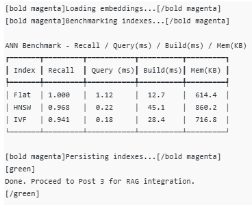
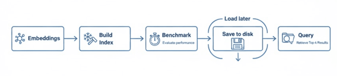 Figure 7: The FAISS index lifecycle — from generating embeddings and building the index to benchmarking, saving for reuse, and querying for top-k results (source: image by the author).
After running the script with:
python 02_vector_search_ann.py --queries 10 --k 5 --ivf-nlist 32 --ivf-nprobe 8 --hnsw-m 32 --hnsw-ef-search 128
FAISS prints a benchmark table comparing Flat, HNSW, and IVF-Flat across recall, query latency, build time, and memory footprint.
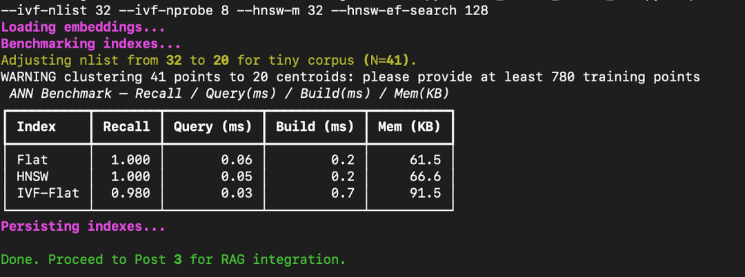 Figure 8: Benchmark results comparing FAISS Flat, HNSW, and IVF-Flat indexes across recall, query latency, build time, and memory usage (source: image by the author).
Let’s break down what this means.
nprobe).Course information:
120+ total classes • 115+ hours hours of on-demand code walkthrough videos • Last updated: August 2026
★★★★★ 4.84 (128 Ratings) • 16,000+ Students Enrolled
I strongly believe that if you had the right teacher you could master computer vision and deep learning.
Do you think learning computer vision and deep learning has to be time-consuming, overwhelming, and complicated? Or has to involve complex mathematics and equations? Or requires a degree in computer science?
That’s not the case.
All you need to master computer vision and deep learning is for someone to explain things to you in simple, intuitive terms. And that’s exactly what I do. My mission is to change education and how complex Artificial Intelligence topics are taught.
If you're serious about learning computer vision, your next stop should be PyImageSearch University, the most comprehensive computer vision, deep learning, and OpenCV course online today. Here you’ll learn how to successfully and confidently apply computer vision to your work, research, and projects. Join me in computer vision mastery.
Inside PyImageSearch University you'll find:
In this tutorial, you moved beyond understanding embeddings and stepped into the practical world of vector search. You began by revisiting the limitations of brute-force similarity search and saw why indexing is crucial when datasets grow larger. Then, you explored how FAISS, Meta’s open-source library for efficient similarity search, builds the backbone of modern vector databases.
From there, you implemented and compared 3 major index types (i.e., Flat, HNSW, and IVF-Flat) each offering a different trade-off between speed, recall, and memory. You wrote code to benchmark their performance, measuring recall@k, query latency, build time, and memory usage, and visualized the results directly in your terminal. Along the way, you saw how HNSW maintains near-perfect accuracy while drastically improving query speed, and how IVF-Flat compresses the search space to achieve sub-millisecond responses even with slight precision loss.
By the end, you not only understood how approximate nearest neighbor (ANN) search works but also saw why it matters — enabling scalable, real-time retrieval without compromising too much on accuracy. You also saved your indexes, preparing them for use in the next lesson, where we’ll connect them to a Retrieval-Augmented Generation (RAG) pipeline and bring everything full circle: embeddings, vector search, and large language models working together in action.
Singh, V. “Vector Search with FAISS: Approximate Nearest Neighbor (ANN) Explained,” PyImageSearch, P. Chugh, S. Huot, A. Sharma, and P. Thakur, eds., 2026, https://pyimg.co/htl5f
@incollection{Singh_2026_vector-search-with-faiss-ann-explained,
  author = {Vikram Singh},
  title = {{Vector Search with FAISS: Approximate Nearest Neighbor (ANN) Explained}},
  booktitle = {PyImageSearch},
  editor = {Puneet Chugh and Susan Huot and Aditya Sharma and Piyush Thakur},
  year = {2026},
  url = {https://pyimg.co/htl5f},
}
To download the source code to this post (and be notified when future tutorials are published here on PyImageSearch), simply enter your email address in the form below!

Enter your email address below to get a .zip of the code and a FREE 17-page Resource Guide on Computer Vision, OpenCV, and Deep Learning. Inside you'll find my hand-picked tutorials, books, courses, and libraries to help you master CV and DL!
| # | Наименование новости | Тональность | Информативность | Дата публикации |
|---|---|---|---|---|
| 1 | Understanding the approximate nearest neighbor (ANN) algorithm | 0 | 8.49 | 17-04-2024 |
| 2 | Vector Search Using Ollama for Retrieval-Augmented Generation (RAG) | 0 | 22.5 | 25-02-2026 |
| 3 | Semantic Caching for LLMs: FastAPI, Redis, and Embeddings | 0 | 10 | 29-04-2026 |
| 4 | DeepSeek-V3 Model: Theory, Config, and Rotary Positional Embeddings | 0 | 22.5 | 12-03-2026 |
| 5 | sentrysearch - Semantic search over videos | 0 | 10 | 26-04-2026 |
| 6 | Алгоритмы векторного поиска: IVF и HNSW | 0 | 7.01 | 16-06-2026 |
| 7 | Векторный поиск в PostgreSQL: PGVector, SQLAlchemy и FastAPI | 0 | 6.31 | 06-03-2026 |
| 8 | Algorithms and SQ Lower Bounds for Robustly Learning Real-valued Multi-Index Models | 0 | 11.59 | 27-08-2026 |
| 9 | The big ideas behind retrieval augmented generation | 0 | 8.98 | 18-09-2024 |
| 10 | Crafting a hybrid geospatial RAG application with Elastic and Amazon Bedrock | 0 | 6.78 | 26-11-2024 |